PDF

Schroeder Diffuser in 2D
Introduction
Sound diffusers are objects or surfaces that are designed to reflect incident sound energy evenly across angles. They are widely used in room acoustics as a way to influence the spatial distribution of the sound field without necessarily attenuating it. One common type of diffuser is the Schroeder diffuser, also called well-based diffuser, which consists of a series of wells of different depths. The depths are determined from a mathematical sequence, such as quadratic residue or primitive root. The principle behind this type of diffuser is that each well will re-emit the incident wave with a different phase shift, causing interferences between the waves emitted by the different wells. The mathematical sequence used to determine the depths of the wells will then dictate the interference pattern and, hence, the polar response of the diffuser.
This model demonstrates how to calculate the scattering coefficient with the Pressure Acoustics, Frequency Domain interface. This coefficient is one of the main inputs for expressing boundary conditions in typical room acoustic simulations. Its measurement procedure can be complicated to set up. Therefore. it is more efficient to determine the data numerically. In addition, the effect of periodicity is investigated by studying the responses from different arrangements of the same diffuser.
Model Definition
The model represents a primitive root diffuser, a type of Schroeder diffuser which aims at eliminating the specular component in the reflected energy polar response (see Ref. 1). The model at hand is based on the primitive root sequence with 7 as odd prime, resulting in a diffuser with six wells. The study is carried out in 2D in order to considerably reduce the number of degrees of freedom in the simulation. Two cases are taken into account as shown in Figure 1:
In the first case, a semicircle with radius r0 = 10 m is added to act as an integration line in the far field. The diffuser and flat reference are surrounded by an air domain terminated by a Perfectly Matched Boundary, and the sound field outside of the calculation domain is obtained from Exterior Field Calculation. In the case of the infinite arrangement, a Periodic Port and Periodic Condition > Floquet periodicity is used to virtually extend the domain in both directions along the x-axis.
A plane wave with incidence angle θ0 from the y-axis is defined as incoming on the diffuser arrangements. The incidence angle is varied in an Auxiliary Sweep from θ0 = 0° to θ0 = 89° with 25 angle steps, resulting in an increment approximately of 3.7°. Frequencies from 50 Hz to 3150 Hz with a third-octave interval are taken into account.
Figure 1: Geometries of the diffuser arrangements. Top left: flat reference; Top right: single diffuser; Bottom: infinite arrangement.
Scattering coefficient
The scattering coefficient s is defined as the power ratio (see Ref. 1)
(1)
with Pspec the power reflected in the specular direction and Ptot the total reflected power. In the infinite arrangement case, Pspec and Ptot are included as built-in variables in the Periodic Port feature, which allows to calculate the scattering coefficient directly. In the case of the single diffuser, the correlation scattering coefficient sc is defined as (see Ref. 1)
(2)
where p0 is the scattered sound pressure from the flat reference, p1 is the scattered sound pressure from the diffuser, and θi is the angle of the ith receiver on the evaluation semicircle Ω with radius r0 located in the far field.
The coefficient in Equation 1 or Equation 2 gives a value for each incidence angle and frequency included in the study. To obtain the random incidence scattering coefficient in octave bands, the Paris formula is used such that (see Ref. 2)
(3)
with θ the incident angle. Although the diffuser studied is asymmetrical, the error due to integrating from 0 to π/2can be tolerated.
Results and Discussion
The sum of incident and scattered sound pressure by the diffuser arrangements and the flat reference is shown in Figure 2 for θ0 = 33.3° and f = 1000 Hz. In this case, the plane waves propagating in the wells of the Schroeder diffuser are clearly visible. Moreover, it is seen that the sound field that would result from a flat solid surface is disrupted by the presence of the wells. This is especially true in front of the diffuser arrangements, where the wavefront tends to a cylindrical wave. It also appears that destructive interferences create directions with greatly reduced energy. Although this effect is present in the single diffuser, it is seen to be more prominent in the infinite arrangement.
Figure 2: Scattered pressure for θ0 = 33.3° and 1000 Hz. Top left: flat reference; Top right: single diffuser; Bottom: infinite arrangement.
Further investigation of the scattered sound field can be made from the SPL polar responses of the single diffuser in Figure 3. It is evaluated in the far field at a distance r0 = 10 m, for θ0 = 33.3° and frequencies around 1000 Hz. This type of plot could not be generated for the infinite arrangement as it requires to evaluate sound pressure on a surrounding semicircle. It can be observed that the primitive root diffuser does reduce the energy reflected in the specular direction as intended. The difference between the SPL in the specular direction and the maximum SPL lies between 10 dB and 25 dB for the single diffuser, with energy being distributed across a few lobes.
Figure 3: Polar response of the single diffuser for θ0 = 33.3° around 1000 Hz.
The scattering coefficients of the two diffuser arrangements are shown in Figure 4 and Figure 5. It is seen that the single diffuser returns similar values to the analytical expression except at 500 Hz. The infinite arrangement also gives interesting results. In this case, the scattering coefficient takes much lower values especially at low frequencies. This is a sign that scattering is dominated by diffraction from the finite size effect at low frequencies, and the wells’ influence is only effective at mid and high frequencies. The values of the scattering coefficients are also tabulated in the model and can be exported.
Figure 4: Random incidence scattering coefficient of the single diffuser.
Figure 5: Random incidence scattering coefficient of the infinite arrangement.
Notes About the COMSOL Implementation
The model is readily set up to investigate a finite arrangement of the Schroeder diffuser. To change the number of periods, simply change the value of the parameter Np in Parameters 2 - Physics and rebuild the geometries for the flat reference and the diffuser.
The infinite arrangement case in this model is set up with the Periodic Port feature. To learn more about how to use this feature, see the Porous Absorber model, also included in the Acoustics Module Application Library.
References
1. T.J. Cox and P. D’Antonio, Acoustics Absorbers and Diffusers: Theory, Design and Application, 2nd edition, Taylor & Francis, 2009.
2. H. Kuttruff, Room Acoustics, 5th edition, CRC Press, 2009.
Application Library path: Acoustics_Module/Building_and_Room_Acoustics/diffuser_schroeder_2d
Modeling Instructions
This section contains the modeling instructions for the Schroeder Diffuser in 2D model. They are followed by the Geometry Modeling Instructions section.
From the File menu, choose New.
New
In the New window, click  Model Wizard.
Model Wizard
1
In the Model Wizard window, click  2D.
2
In the Select Physics tree, select Acoustics > Pressure Acoustics > Pressure Acoustics, Frequency Domain (acpr).
3
Click Add.
4
Click  Study.
5
In the Select Study tree, select General Studies > Frequency Domain.
6
Start by importing the geometry cases and the parameters needed for the study.
Flat Reference
1
In the Model Builder window, click Component 1 (comp1).
2
In the Settings window for Component, type Flat Reference in the Label text field.
Geometry 1
1
In the Geometry toolbar, click Insert Sequence and choose Insert Sequence.
2
3
In the Insert Sequence dialog, select Geometry 3 in the Select geometry sequence to insert list.
4
1
In the Model Builder window, under Flat Reference (comp1) click Geometry 1.
2
In the Geometry toolbar, click  Build All.
Add Component
Right-click Flat Reference (comp1) > Geometry 1 and choose Add Component > 2D.
Single Diffuser
In the Settings window for Component, type Single Diffuser in the Label text field.
Geometry 2
1
In the Geometry toolbar, click Insert Sequence and choose Insert Sequence.
2
3
In the Insert Sequence dialog, select Geometry 2 in the Select geometry sequence to insert list.
4
1
In the Model Builder window, under Single Diffuser (comp2) click Geometry 2.
2
In the Geometry toolbar, click  Build All.
Add Component
Right-click Single Diffuser (comp2) > Geometry 2 and choose Add Component > 2D.
Infinite Arrangement
In the Settings window for Component, type Infinite Arrangement in the Label text field.
Geometry 3
1
In the Geometry toolbar, click Insert Sequence and choose Insert Sequence.
2
3
In the Insert Sequence dialog, click OK.
1
In the Model Builder window, under Infinite Arrangement (comp3) click Geometry 3.
2
In the Geometry toolbar, click  Build All.
Add Material
1
In the Materials toolbar, click  Add Material to open the Add Material window.
2
Go to the Add Material window.
3
In the tree, select Built-in > Air.
4
Click the right end of the Add to Component split button in the window toolbar.
5
From the menu, choose Add to Flat Reference (comp1).
6
Click the Add to Single Diffuser (comp2) button in the window toolbar.
7
Click the Add to Infinite Arrangement (comp3) button in the window toolbar.
8
In the Materials toolbar, click  Add Material to close the Add Material window.
Global Definitions
Parameters 1 - Geometry
1
In the Model Builder window, under Global Definitions click Parameters 1.
2
In the Settings window for Parameters, type Parameters 1 - Geometry in the Label text field.
Parameters 2 - Physics
1
In the Home toolbar, click  Parameters and choose Add > Parameters.
2
In the Settings window for Parameters, type Parameters 2 - Physics in the Label text field.
3
Locate the Parameters section. Click  Load from File.
4
Proceed with setting up the physics and local variables for the flat reference and single diffuser.
Pressure Acoustics, Frequency Domain (acpr)
In the Model Builder window, under Flat Reference (comp1) click Pressure Acoustics, Frequency Domain (acpr).
Background Pressure Field 1
1
In the Physics toolbar, click  Domains and choose Background Pressure Field.
2
In the Settings window for Background Pressure Field, locate the Domain Selection section.
3
From the Selection list, choose All domains.
4
Locate the Background Pressure Field section. In the p0 text field, type p0.
5
In the c text field, type c0.
6
Specify the ek vector as
Perfectly Matched Boundary 1
1
In the Physics toolbar, click  Boundaries and choose Perfectly Matched Boundary.
2
Exterior Field Calculation 1
1
In the Physics toolbar, click  Boundaries and choose Exterior Field Calculation.
2
Interior Sound Hard Boundary (Wall) 1
1
In the Physics toolbar, click  Boundaries and choose Interior Sound Hard Boundary (Wall).
2
Single Diffuser (comp2)
In the Model Builder window, click Single Diffuser (comp2).
Add Physics
1
In the Home toolbar, click  Add Physics to open the Add Physics window.
2
Go to the Add Physics window.
3
In the tree, select Acoustics > Pressure Acoustics > Pressure Acoustics, Frequency Domain (acpr).
4
Click the Add to Single Diffuser button in the window toolbar.
5
In the Home toolbar, click  Add Physics to close the Add Physics window.
Definitions (comp2)
Integration 1 (intop1)
1
In the Definitions toolbar, click  Nonlocal Couplings and choose Integration.
2
In the Settings window for Integration, locate the Source Selection section.
3
From the Geometric entity level list, choose Boundary.
4
Variables 1
1
In the Model Builder window, right-click Definitions and choose Variables.
2
In the Settings window for Variables, locate the Variables section.
3
Click  Load from File.
4
Pressure Acoustics, Frequency Domain 2 (acpr2)
Background Pressure Field 1
1
In the Physics toolbar, click  Domains and choose Background Pressure Field.
2
In the Settings window for Background Pressure Field, locate the Domain Selection section.
3
From the Selection list, choose All domains.
4
Locate the Background Pressure Field section. In the p0 text field, type p0.
5
In the c text field, type c0.
6
Specify the ek vector as
Perfectly Matched Boundary 1
1
In the Physics toolbar, click  Boundaries and choose Perfectly Matched Boundary.
2
Exterior Field Calculation 1
1
In the Physics toolbar, click  Boundaries and choose Exterior Field Calculation.
2
Interior Sound Hard Boundary (Wall) 1
1
In the Physics toolbar, click  Boundaries and choose Interior Sound Hard Boundary (Wall).
2
In the Settings window for Interior Sound Hard Boundary (Wall), locate the Boundary Selection section.
3
From the Selection list, choose Array 1.
Set up the study to calculate the single diffuser and its corresponding flat reference.
Study 1 - Single Diffuser
1
In the Model Builder window, click Study 1.
2
In the Settings window for Study, type Study 1 - Single Diffuser in the Label text field.
Step 1: Frequency Domain
1
In the Model Builder window, under Study 1 - Single Diffuser click Step 1: Frequency Domain.
2
In the Settings window for Frequency Domain, locate the Study Settings section.
3
Click  Range.
4
In the Range dialog, choose ISO preferred frequencies from the Entry method list.
5
In the Start frequency text field, type fmin.
6
In the Stop frequency text field, type fmax.
7
From the Interval list, choose 1/3 octave.
8
Click Replace.
9
In the Settings window for Frequency Domain, locate the Physics and Variables Selection section.
10
In the Solve for column of the table, clear the checkbox for Infinite Arrangement (comp3).
11
Click to expand the Study Extensions section. Select the Auxiliary sweep checkbox.
12
13
Generate the mesh based on the Physics-controlled mesh suggestion. The frequency controlling the maximum element size is per default taken From study, that is, from the Maximum frequency to resolve. In general, 5 to 6 second-order elements per wavelength are needed to resolve the waves. For more details, see Meshing (Resolving the Waves) in the Acoustics Module User’s Guide. In this model, use the default Automatic option, which gives 5 elements per wavelength. An Edge mesh is then added on the circular arc.
Mesh 1
In the Model Builder window, under Flat Reference (comp1) right-click Mesh 1 and choose Build All.
Mesh 2
1
In the Model Builder window, under Single Diffuser (comp2) click Mesh 2.
2
In the Settings window for Mesh, locate the Sequence Type section.
3
From the list, choose User-controlled mesh.
Edge 1
1
In the Mesh toolbar, click  More Generators and choose Edge.
2
Distribution 1
1
Right-click Edge 1 and choose Distribution.
2
In the Settings window for Distribution, locate the Distribution section.
3
In the Number of elements text field, type 100.
Free Triangular 1
1
In the Model Builder window, under Single Diffuser (comp2) > Mesh 2 click Free Triangular 1.
2
In the Settings window for Free Triangular, locate the Domain Selection section.
3
From the Geometric entity level list, choose Domain.
4
From the Selection list, choose All domains.
5
In the Model Builder window, right-click Mesh 2 and choose Build All.
Define the third component with a Periodic Condition to model an infinite arrangement of diffusers. As a consequence, the sound pressure in the exterior field cannot be evaluated on a circular arc in this case; the calculation of the energy reflected in the specular direction is thus based on a Periodic Port.
Infinite Arrangement (comp3)
In the Model Builder window, click Infinite Arrangement (comp3).
Add Physics
1
In the Home toolbar, click  Add Physics to open the Add Physics window.
2
Go to the Add Physics window.
3
In the tree, select Acoustics > Pressure Acoustics > Pressure Acoustics, Frequency Domain (acpr).
4
Click the Add to Infinite Arrangement button in the window toolbar.
5
In the Home toolbar, click  Add Physics to close the Add Physics window.
Definitions (comp3)
Variables 2
1
In the Model Builder window, under Infinite Arrangement (comp3) right-click Definitions and choose Variables.
2
In the Settings window for Variables, locate the Variables section.
3
Click  Load from File.
4
Set up the Periodic Port. It must include all the propagating diffraction orders in order to be correct.
Pressure Acoustics, Frequency Domain 3 (acpr3)
Periodic Port 1
1
In the Physics toolbar, click  Boundaries and choose Periodic Port.
2
3
In the Settings window for Periodic Port, locate the Port Mode Settings section.
4
From the Define incident wave list, choose Power per unit length.
5
In the Pin text field, type 1.
6
In the θin text field, type theta0.
Diffraction Order Port 1
1
In the Physics toolbar, click  Attributes and choose Diffraction Order Port.
2
In the Settings window for Diffraction Order Port, locate the Diffraction Order Port section.
3
In the m text field, type 1.
Repeat this operation for all the diffraction orders needed.
Periodic Condition 1
1
In the Physics toolbar, click  Boundaries and choose Periodic Condition.
2
3
In the Settings window for Periodic Condition, locate the Periodicity Settings section.
4
From the Type of periodicity list, choose Floquet periodicity.
5
From the kF list, choose Periodic port Floquet wave number vector (acpr3/pport1).
Proceed with setting up the study.
Add Study
1
In the Home toolbar, click  Add Study to open the Add Study window.
2
Go to the Add Study window.
3
Find the Studies subsection. In the Select Study tree, select General Studies > Frequency Domain.
4
Click the Add Study button in the window toolbar.
5
In the Home toolbar, click  Add Study to close the Add Study window.
Study 2 - Infinite arrangement
1
In the Settings window for Study, type Study 2 - Infinite arrangement in the Label text field.
2
Locate the Study Settings section. Clear the Generate default plots checkbox.
Step 1: Frequency Domain
1
In the Model Builder window, under Study 2 - Infinite arrangement click Step 1: Frequency Domain.
2
In the Settings window for Frequency Domain, locate the Study Settings section.
3
Click  Range.
4
In the Range dialog, choose ISO preferred frequencies from the Entry method list.
5
In the Start frequency text field, type fmin.
6
In the Stop frequency text field, type fmax.
7
From the Interval list, choose 1/3 octave.
8
Click Replace.
9
In the Settings window for Frequency Domain, locate the Physics and Variables Selection section.
10
In the Solve for column of the table, clear the checkboxes for Flat Reference (comp1) and Single Diffuser (comp2).
11
Locate the Study Extensions section. Select the Auxiliary sweep checkbox.
12
13
Mesh 3
In the Model Builder window, under Infinite Arrangement (comp3) right-click Mesh 3 and choose Build All.
Now solve the two studies.
Study 1 - Single Diffuser
In the Home toolbar, click  Compute.
Study 2 - Infinite arrangement
Click  Compute.
Results
1
In the Model Builder window, click Results.
2
In the Settings window for Results, locate the Update of Results section.
3
Select the Only plot when requested checkbox.
Before investigating the results, remove the circular arc from the datasets. It only serves a purpose for calculating integrals and does not need to be shown in the result plots. Also remove unnecessary datasets and duplicate default plots.
In the Model Builder window, expand the Results > Datasets node.
Study 1 - Single Diffuser/Solution 1 (3) (sol1), Study 2 - Infinite arrangement/Solution 2 (4) (sol2), Study 2 - Infinite arrangement/Solution 2 (5) (sol2)
1
In the Model Builder window, under Results > Datasets, Ctrl-click to select Study 1 - Single Diffuser/Solution 1 (3) (sol1), Study 2 - Infinite arrangement/Solution 2 (4) (sol2), and Study 2 - Infinite arrangement/Solution 2 (5) (sol2).
2
Study 1 - Single Diffuser/Solution 1 (2) (sol1)
In the Model Builder window, under Results > Datasets click Study 1 - Single Diffuser/Solution 1 (2) (sol1).
Selection
1
Right-click Study 1 - Single Diffuser/Solution 1 (2) (sol1) and choose Selection.
2
In the Settings window for Selection, locate the Geometric Entity Selection section.
3
From the Geometric entity level list, choose Domain.
4
From the Selection list, choose All domains.
Create an Array dataset to show multiple periods of the infinite arrangement of diffusers.
Array 2D - 5 periods of the infinite arrangement
1
In the Results toolbar, click  More Datasets and choose Array 2D.
2
In the Settings window for Array 2D, locate the Data section.
3
From the Dataset list, choose Study 2 - Infinite arrangement/Solution 2 (sol2).
4
In the Label text field, type Array 2D - 5 periods of the infinite arrangement.
5
Locate the Array Size section. In the X size text field, type 5.
6
Click to expand the Advanced section. Select the Floquet–Bloch periodicity checkbox.
7
Find the Wave vector subsection. In the X text field, type acpr3.pport1.kitx.
8
In the Y text field, type acpr3.pport1.kity.
Acoustic Pressure (acpr2), Exterior-Field Pressure (acpr2), Exterior-Field Sound Pressure Level (acpr2), Sound Pressure Level (acpr2)
1
In the Model Builder window, under Results, Ctrl-click to select Acoustic Pressure (acpr2), Sound Pressure Level (acpr2), Exterior-Field Sound Pressure Level (acpr2), and Exterior-Field Pressure (acpr2).
2
Acoustic Pressure (acpr)
1
In the Model Builder window, under Results click Acoustic Pressure (acpr).
2
In the Settings window for 2D Plot Group, locate the Data section.
3
From the Parameter value (freq (Hz)) list, choose 1000.
4
From the Parameter value (theta0 (deg)) list, choose 33.375.
5
In the Acoustic Pressure (acpr) toolbar, click  Plot.
6
Click the  Zoom Extents button in the Graphics toolbar.
7
In the Model Builder window, click Acoustic Pressure (acpr).
8
From the Dataset list, choose Study 1 - Single Diffuser/Solution 1 (2) (sol1).
Surface 1
1
In the Model Builder window, expand the Acoustic Pressure (acpr) node, then click Surface 1.
2
In the Settings window for Surface, locate the Expression section.
3
In the Expression text field, type acpr2.p_t.
4
In the Acoustic Pressure (acpr) toolbar, click  Plot.
5
Click the  Zoom Extents button in the Graphics toolbar.
Acoustic Pressure (acpr)
1
In the Model Builder window, click Acoustic Pressure (acpr).
2
In the Settings window for 2D Plot Group, locate the Data section.
3
From the Dataset list, choose Array 2D - 5 periods of the infinite arrangement.
Surface 1
1
In the Model Builder window, click Surface 1.
2
In the Settings window for Surface, locate the Expression section.
3
In the Expression text field, type acpr3.p_t.
4
In the Acoustic Pressure (acpr) toolbar, click  Plot.
5
Click the  Zoom Extents button in the Graphics toolbar.
Sound Pressure Level (acpr)
1
In the Model Builder window, under Results click Sound Pressure Level (acpr).
2
In the Settings window for 2D Plot Group, locate the Data section.
3
From the Dataset list, choose Array 2D - 5 periods of the infinite arrangement.
4
From the Parameter value (freq (Hz)) list, choose 1000.
5
From the Parameter value (theta0 (deg)) list, choose 33.375.
Surface 1
1
In the Model Builder window, expand the Sound Pressure Level (acpr) node, then click Surface 1.
2
In the Settings window for Surface, locate the Expression section.
3
In the Expression text field, type acpr3.Lp_t.
4
In the Sound Pressure Level (acpr) toolbar, click  Plot.
5
Click the  Zoom Extents button in the Graphics toolbar.
Exterior-Field Sound Pressure Level (acpr)
1
In the Model Builder window, under Results click Exterior-Field Sound Pressure Level (acpr).
2
In the Settings window for Polar Plot Group, locate the Data section.
3
From the Dataset list, choose Study 1 - Single Diffuser/Solution 1 (2) (sol1).
4
From the Parameter selection (freq) list, choose From list.
5
In the Parameter values (freq (Hz)) list, choose 630, 800, 1000, and 1250.
6
From the Parameter selection (theta0) list, choose From list.
7
In the Parameter values (theta0 (deg)) list box, select 33.375.
8
Locate the Axis section. Select the Symmetric angle range checkbox.
9
From the Zero angle list, choose Up.
10
Locate the Legend section. From the Position list, choose Manual.
11
In the x-position text field, type 0.5.
12
In the y-position text field, type 0.25.
Radiation Pattern 1
1
In the Model Builder window, expand the Exterior-Field Sound Pressure Level (acpr) node, then click Radiation Pattern 1.
2
In the Settings window for Radiation Pattern, locate the Expression section.
3
In the Expression text field, type acpr2.efc1.Lp_pext.
4
Locate the Evaluation section. Find the Angles subsection. In the Number of angles text field, type 360.
5
From the Restriction list, choose Manual.
6
In the ϕ start text field, type -90.
7
In the ϕ range text field, type 180.
8
Find the Circle subsection. From the Circle list, choose Manual.
9
Find the Evaluation distance subsection. In the Radius text field, type r0.
10
Find the Reference direction subsection. In the x text field, type 0.
11
In the y text field, type 1.
12
In the Exterior-Field Sound Pressure Level (acpr) toolbar, click  Plot.
Exterior-Field Pressure (acpr)
1
In the Model Builder window, under Results click Exterior-Field Pressure (acpr).
2
In the Settings window for Polar Plot Group, locate the Data section.
3
From the Dataset list, choose Study 1 - Single Diffuser/Solution 1 (2) (sol1).
4
From the Parameter selection (freq) list, choose From list.
5
In the Parameter values (freq (Hz)) list, choose 630, 800, 1000, and 1250.
6
From the Parameter selection (theta0) list, choose From list.
7
In the Parameter values (theta0 (deg)) list box, select 40.792.
8
Locate the Axis section. Select the Symmetric angle range checkbox.
9
From the Zero angle list, choose Up.
10
Locate the Legend section. From the Position list, choose Manual.
11
In the x-position text field, type 0.5.
12
In the y-position text field, type 0.25.
Radiation Pattern 1
1
In the Model Builder window, expand the Exterior-Field Pressure (acpr) node, then click Radiation Pattern 1.
2
In the Settings window for Radiation Pattern, locate the Expression section.
3
In the Expression text field, type abs(acpr2.efc1.pext)^2.
4
In the Unit field, type Pa^2.
5
Select the Description checkbox. In the associated text field, type Exterior-field sound energy.
6
Locate the Evaluation section. Find the Angles subsection. In the Number of angles text field, type 360.
7
From the Restriction list, choose Manual.
8
In the ϕ start text field, type -90.
9
In the ϕ range text field, type 180.
10
Find the Circle subsection. From the Circle list, choose Manual.
11
Find the Evaluation distance subsection. In the Radius text field, type r0.
12
Find the Reference direction subsection. In the x text field, type 0.
13
In the y text field, type 1.
14
In the Exterior-Field Pressure (acpr) toolbar, click  Plot.
Scattering from Single Diffuser
In the Home toolbar, click  Add Plot Group and choose 1D Plot Group.
Plot the scattering coefficients for the single diffuser and the infinite arrangement. The Octave Band plots automatically create tables to easily export data.
1
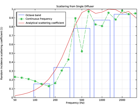
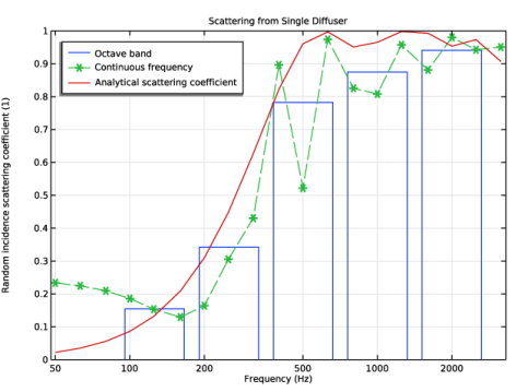
In the Settings window for 1D Plot Group, type Scattering from Single Diffuser in the Label text field.
2
Locate the Data section. From the Dataset list, choose Study 1 - Single Diffuser/Solution 1 (2) (sol1).
3
From the Parameter selection (theta0) list, choose First.
4
Click to expand the Title section. From the Title type list, choose Label.
5
Locate the Plot Settings section.
6
Select the x-axis label checkbox. In the associated text field, type Frequency (Hz).
7
Select the y-axis label checkbox. In the associated text field, type Random incidence scattering coefficient (1).
8
Locate the Axis section. Select the Manual axis limits checkbox.
9
In the x minimum text field, type 48.
10
In the x maximum text field, type 3300.
11
In the y minimum text field, type 0.
12
Select the x-axis log scale checkbox.
13
Locate the Legend section. From the Position list, choose Upper left.
Octave Band 1
1
In the Scattering from Single Diffuser toolbar, click  More Plots and choose Octave Band.
2
In the Settings window for Octave Band, locate the Selection section.
3
From the Geometric entity level list, choose Global.
4
Locate the y-Axis Data section. In the Expression text field, type s_ran.
5
From the Expression type list, choose General (non-dB).
6
Locate the Plot section. From the Quantity list, choose Band average power spectral density.
7
Click to expand the Coloring and Style section. From the Type list, choose Outline.
8
Click to expand the Legends section. Select the Show legends checkbox.
9
From the Legends list, choose Manual.
10
Octave Band 2
1
Right-click Octave Band 1 and choose Duplicate.
2
In the Settings window for Octave Band, locate the Plot section.
3
From the Quantity list, choose Continuous power spectral density.
4
Locate the Coloring and Style section. Find the Line style subsection. From the Line list, choose Dashed.
5
Find the Line markers subsection. From the Marker list, choose Asterisk.
6
Locate the Legends section. In the table, enter the following settings:
Global 1
1
In the Model Builder window, right-click Scattering from Single Diffuser and choose Global.
2
In the Settings window for Global, locate the Data section.
3
From the Dataset list, choose Study 2 - Infinite arrangement/Solution 2 (sol2).
4
From the Parameter selection (theta0) list, choose First.
5
Locate the y-Axis Data section. In the table, enter the following settings:
6
Locate the x-Axis Data section. From the Axis source data list, choose freq.
7
Click to expand the Legends section. Find the Include subsection. Clear the Solution checkbox.
Before plotting, note that the single diffuser case may take a long time to render. The infinite arrangement case is much faster thanks to the Periodic Port setup
In the Scattering from Single Diffuser toolbar, click  Plot.
Scattering from Infinite Arrangement
1
Right-click Scattering from Single Diffuser and choose Duplicate.
2
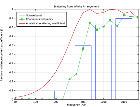
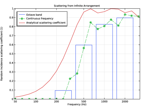
In the Settings window for 1D Plot Group, type Scattering from Infinite Arrangement in the Label text field.
3
Locate the Data section. From the Dataset list, choose Study 2 - Infinite arrangement/Solution 2 (sol2).
4
In the Scattering from Infinite Arrangement toolbar, click  Plot.
Periodic Port Mode Powers
In the Home toolbar, click  Add Plot Group and choose 1D Plot Group.
Investigate the behavior of the Periodic Port by plotting the powers of the diffraction orders.
1
In the Settings window for 1D Plot Group, type Periodic Port Mode Powers in the Label text field.
2
Locate the Data section. From the Dataset list, choose Study 2 - Infinite arrangement/Solution 2 (sol2).
3
From the Parameter selection (freq) list, choose Last.
4
Click to expand the Title section. From the Title type list, choose Label.
5
Locate the Plot Settings section.
6
Select the x-axis label checkbox. In the associated text field, type Incidence angle (deg).
7
Select the y-axis label checkbox. In the associated text field, type Power per unit length (W/m).
8
Locate the Legend section. From the Position list, choose Middle left.
Global 1
1
Right-click Periodic Port Mode Powers and choose Global.
2
In the Settings window for Global, locate the y-Axis Data section.
3
4
Click to expand the Coloring and Style section. Find the Line markers subsection. From the Marker list, choose Point.
5
Click to expand the Legends section. From the Legends list, choose Manual.
6
Global 2
1
In the Model Builder window, right-click Periodic Port Mode Powers and choose Global.
2
In the Settings window for Global, locate the y-Axis Data section.
3
4
Locate the Legends section. Clear the Show legends checkbox.
Global 3
1
Right-click Periodic Port Mode Powers and choose Global.
2
In the Settings window for Global, locate the y-Axis Data section.
3
4
Locate the Coloring and Style section. Find the Line style subsection. From the Line list, choose Dashed.
5
Locate the Legends section. Clear the Show legends checkbox.
6
In the Periodic Port Mode Powers toolbar, click  Plot.
Evaluation Group 1 - Propagating Diffraction Orders
In the Results toolbar, click  Evaluation Group.
To make sure that all the propagating modes have been included in the Periodic Port, evaluate the imaginary part of the mode wave number for each diffraction order.
1
In the Settings window for Evaluation Group, type Evaluation Group 1 - Propagating Diffraction Orders in the Label text field.
2
Locate the Data section. From the Dataset list, choose Study 2 - Infinite arrangement/Solution 2 (sol2).
3
From the Parameter selection (freq) list, choose Last.
Global Evaluation 1
1
Right-click Evaluation Group 1 - Propagating Diffraction Orders and choose Global Evaluation.
2
In the Settings window for Global Evaluation, locate the Expressions section.
3
4
In the Evaluation Group 1 - Propagating Diffraction Orders toolbar, click  Evaluate.
Geometry Modeling Instructions
From the File menu, choose New.
New
In the New window, click  Blank Model.
Global Definitions
Parameters 1
1
In the Model Builder window, under Global Definitions click Parameters 1.
2
In the Settings window for Parameters, locate the Parameters section.
3
Click  Load from File.
4
Add Component
In the Home toolbar, click  Add Component and choose 2D.
Infinite arrangement
1
In the Model Builder window, click Component 1 (comp1).
2
In the Settings window for Component, type Infinite arrangement in the Label text field.
Geometry 1
Rectangle 1 (r1)
1
In the Geometry toolbar, click  Rectangle.
2
In the Settings window for Rectangle, locate the Size and Shape section.
3
In the Width text field, type W.
4
In the Height text field, type d1.
5
In the Width text field, type Lw.
6
Locate the Position section. In the x text field, type -L/2+Li/2.
7
In the y text field, type -d1.
Rectangle 2 (r2)
1
In the Geometry toolbar, click  Rectangle.
2
In the Settings window for Rectangle, locate the Size and Shape section.
3
In the Width text field, type Lw.
4
In the Height text field, type d2.
5
Locate the Position section. In the x text field, type -L/2+3*Li/2+Lw.
6
In the y text field, type -d2.
Rectangle 3 (r3)
1
In the Geometry toolbar, click  Rectangle.
2
In the Settings window for Rectangle, locate the Size and Shape section.
3
In the Width text field, type Lw.
4
In the Height text field, type d3.
5
Locate the Position section. In the x text field, type -L/2+5*Li/2+2*Lw.
6
In the y text field, type -d3.
Rectangle 4 (r4)
1
In the Geometry toolbar, click  Rectangle.
2
In the Settings window for Rectangle, locate the Size and Shape section.
3
In the Width text field, type Lw.
4
In the Height text field, type d4.
5
Locate the Position section. In the x text field, type -L/2+7*Li/2+3*Lw.
6
In the y text field, type -d4.
Rectangle 5 (r5)
1
In the Geometry toolbar, click  Rectangle.
2
In the Settings window for Rectangle, locate the Size and Shape section.
3
In the Width text field, type Lw.
4
In the Height text field, type d5.
5
Locate the Position section. In the x text field, type -L/2+9*Li/2+4*Lw.
6
In the y text field, type -d5.
Rectangle 6 (r6)
1
In the Geometry toolbar, click  Rectangle.
2
In the Settings window for Rectangle, locate the Size and Shape section.
3
In the Width text field, type Lw.
4
In the Height text field, type d6.
5
Locate the Position section. In the x text field, type -L/2+11*Li/2+5*Lw.
6
In the y text field, type -d6.
Rectangle 1 (r1), Rectangle 2 (r2), Rectangle 3 (r3), Rectangle 4 (r4), Rectangle 5 (r5), Rectangle 6 (r6)
1
In the Model Builder window, under Infinite arrangement (comp1) > Geometry 1, Ctrl-click to select Rectangle 1 (r1), Rectangle 2 (r2), Rectangle 3 (r3), Rectangle 4 (r4), Rectangle 5 (r5), and Rectangle 6 (r6).
2
Wells
In the Settings window for Group, type Wells in the Label text field.
Rectangle 7 (r7)
1
In the Geometry toolbar, click  Rectangle.
2
In the Settings window for Rectangle, locate the Size and Shape section.
3
In the Width text field, type L.
4
In the Height text field, type Hair.
5
Locate the Position section. In the x text field, type -L/2.
Union 1 (uni1)
1
In the Geometry toolbar, click  Booleans and Partitions and choose Union.
2
Click in the Graphics window and then press Ctrl+A to select all objects.
3
In the Settings window for Union, locate the Union section.
4
Clear the Keep interior boundaries checkbox.
5
In the Geometry toolbar, click  Build All.
6
Click the  Zoom Extents button in the Graphics toolbar.
7
In the Model Builder window, click Geometry 1.
Add Component
Right-click Geometry 1 and choose Add Component > 2D.
Single Diffuser
In the Settings window for Component, type Single Diffuser in the Label text field.
Geometry 1
Wells
In the Model Builder window, under Infinite arrangement (comp1) > Geometry 1 right-click Wells and choose Copy.
Geometry 2
In the Model Builder window, under Single Diffuser (comp2) right-click Geometry 2 and choose Paste Group.
Line Segment 1 (ls1)
1
In the Geometry toolbar, click  More Primitives and choose Line Segment.
2
In the Settings window for Line Segment, locate the Starting Point section.
3
From the Specify list, choose Coordinates.
4
In the x text field, type -L/2.
5
Locate the Endpoint section. From the Specify list, choose Coordinates.
6
In the x text field, type -L/2+Li/2.
Line Segment 2 (ls2)
1
In the Geometry toolbar, click  More Primitives and choose Line Segment.
2
In the Settings window for Line Segment, locate the Starting Point section.
3
Click to select the  Activate Selection toggle button for Start vertex.
4
On the object r1, select Point 3 only.
5
Locate the Endpoint section. Click to select the  Activate Selection toggle button for End vertex.
6
On the object r2, select Point 4 only.
Line Segment 3 (ls3)
1
In the Geometry toolbar, click  More Primitives and choose Line Segment.
2
On the object r2, select Point 3 only.
3
In the Settings window for Line Segment, locate the Endpoint section.
4
Click to select the  Activate Selection toggle button for End vertex.
5
On the object r3, select Point 4 only.
Line Segment 4 (ls4)
1
In the Geometry toolbar, click  More Primitives and choose Line Segment.
2
On the object r3, select Point 3 only.
3
In the Settings window for Line Segment, locate the Endpoint section.
4
Click to select the  Activate Selection toggle button for End vertex.
5
On the object r4, select Point 4 only.
Line Segment 5 (ls5)
1
In the Geometry toolbar, click  More Primitives and choose Line Segment.
2
On the object r4, select Point 3 only.
3
In the Settings window for Line Segment, locate the Endpoint section.
4
Click to select the  Activate Selection toggle button for End vertex.
5
On the object r5, select Point 4 only.
Line Segment 6 (ls6)
1
In the Geometry toolbar, click  More Primitives and choose Line Segment.
2
On the object r5, select Point 3 only.
3
In the Settings window for Line Segment, locate the Endpoint section.
4
Click to select the  Activate Selection toggle button for End vertex.
5
On the object r6, select Point 4 only.
Line Segment 7 (ls7)
1
In the Geometry toolbar, click  More Primitives and choose Line Segment.
2
In the Settings window for Line Segment, locate the Starting Point section.
3
From the Specify list, choose Coordinates.
4
In the x text field, type L/2-Li/2.
5
Locate the Endpoint section. From the Specify list, choose Coordinates.
6
In the x text field, type L/2.
Delete Entities 1 (del1)
1
In the Model Builder window, right-click Geometry 2 and choose Delete Entities.
2
On the object r1, select Boundary 3 only.
3
On the object r2, select Boundary 3 only.
4
On the object r3, select Boundary 3 only.
5
On the object r4, select Boundary 3 only.
6
On the object r5, select Boundary 3 only.
7
On the object r6, select Boundary 3 only.
Array 1 (arr1)
1
In the Geometry toolbar, click  Transforms and choose Array.
2
In the Settings window for Array, locate the Input section.
3
From the Input objects list, choose All objects.
4
Locate the Size section. In the x size text field, type Np.
5
Locate the Displacement section. In the x text field, type L.
6
Locate the Selections of Resulting Entities section. Select the Resulting objects selection checkbox.
7
From the Show in physics list, choose Boundary selection.
Move 1 (mov1)
1
In the Geometry toolbar, click  Transforms and choose Move.
2
In the Settings window for Move, locate the Input section.
3
From the Input objects list, choose All objects.
4
Locate the Displacement section. In the x text field, type -(Np-1)*L/2.
Rectangle 7 (r7)
1
In the Geometry toolbar, click  Rectangle.
2
In the Settings window for Rectangle, locate the Size and Shape section.
3
In the Width text field, type Wair.
4
In the Height text field, type 2*Hair.
5
Locate the Position section. From the Base list, choose Center.
Union 1 (uni1)
1
In the Geometry toolbar, click  Booleans and Partitions and choose Union.
2
In the Settings window for Union, locate the Union section.
3
From the Input objects list, choose All objects.
4
In the Geometry toolbar, click  Build All.
5
Click the  Zoom Extents button in the Graphics toolbar.
6
In the Model Builder window, click Geometry 2.
Circular Arc 1 (ca1)
1
In the Geometry toolbar, click  More Primitives and choose Circular Arc.
2
In the Settings window for Circular Arc, locate the Radius section.
3
In the Radius text field, type r0.
4
Locate the Angles section. In the End angle text field, type 180.
5
In the Geometry toolbar, click  Build All.
Add Component
Right-click Geometry 2 and choose Add Component > 2D.
Flat Reference
In the Settings window for Component, type Flat Reference in the Label text field.
Geometry 2
Rectangle 7 (r7)
In the Model Builder window, under Single Diffuser (comp2) > Geometry 2 right-click Rectangle 7 (r7) and choose Copy.
Geometry 3
Rectangle 7 (r1)
In the Model Builder window, under Flat Reference (comp3) right-click Geometry 3 and choose Paste Rectangle.
Line Segment 1 (ls1)
1
In the Geometry toolbar, click  More Primitives and choose Line Segment.
2
In the Settings window for Line Segment, locate the Starting Point section.
3
From the Specify list, choose Coordinates.
4
In the x text field, type -Np*L/2.
5
Locate the Endpoint section. From the Specify list, choose Coordinates.
6
In the x text field, type Np*L/2.
7
In the Geometry toolbar, click  Build All.
8
Click the  Zoom Extents button in the Graphics toolbar.
9
In the Model Builder window, click Geometry 3.