PDF

Axisymmetric Condenser Microphone
Introduction
This is a model of a condenser microphone with a simple axisymmetric geometry. The model aims to give a precise description of the physical working principles of such a microphone. The simulation results in the sensitivity curve of the transducer, that is, the transformation from detected pressure to measured voltage. The model also predicts the DC and AC capacitance of the microphone.
The condenser microphone is considered to be the microphone with highest quality when performing precise acoustical measurements and with high-fidelity reproduction properties when performing sound recordings; see Ref. 2. This electromechanical acoustic transducer works by transforming the mechanical deformation of a thin membrane (diaphragm) into an AC voltage signal.
Figure 1: Sketch of the condenser microphone system (axisymmetric geometry) including variables and coordinate system.
Models for describing condenser microphones have classically been of the equivalent network type; see Ref. 2. Analytical models exist for simpler geometries, but there are also highly advanced analytical models for more complex geometries; see for example Ref. 1 or Ref. 4. In the present detailed finite-element model, the thermoviscous acoustic, electric, and structural problem is solved fully coupled using the frequency-domain linear perturbation solver. This includes the DC charging (prepolarization) and deformation of the membrane which makes out the zeroth order linearization point. A small external circuit model is added to model the preamplifier (voltage source and resistor) connected to the terminal. In some cases, lumping of the electrical part is a good approximation, especially for simple geometries such as this one, where the back electrode is flat and has no perforations. During the initial design steps, lumped models are an important tool. In more complex geometries, solving the full set of equations is necessary to get the correct response.
Theoretical Membrane Model
In order to compare the results of the simulation, the model uses the analytical solution derived for an undamped axisymmetric membrane. The displacement U of a thin axisymmetric membrane of thickness tm, under constant tension Tm, and with a density ρm is governed by the following equation
(1)
where r is the radial coordinate, t is time, ρms = ρm/tm is the surface density, and Fs is the sum of surface forces; see for example Ref. 3. In the present model, the surface force is the sum of the external incident pressure pin (it is assumed to be uniform over the microphone membrane), the internal pressure p = p(r) (given by the thermoviscous acoustics model), and the electrostatic force which is the sum of the quiescent Maxwell surface stress n ⋅ τ (given by the electrostatic model) and the small-signal force fes. The variation of the deformation U is assumed to be small and harmonic on top of the static contribution U0 from the DC polarization, such that
(2)
Using these expressions, Equation 1 is reformulated into a static and a time-harmonic equation as
(3)
The latter equation may be rewritten in terms of the axial velocity, um = iωU, of the membrane in the form of a Helmholtz equation:
(4)
Here km is the membrane wave number. In this model, you disregard the change in tension due to the movement of the membrane, which is a nonlinear effect that is small compared to the tension Tm.
The current model represents a true multiphysics problem that involves several physics interfaces: Thermoviscous Acoustics, Electrostatics, Electrical Circuit, a Membrane model and the Moving Mesh feature. The analytical solution of the above equation is shown for comparison in the results section.
Note: This application requires the AC/DC Module and the Structural Mechanics Module in addition to the Acoustics Module.
Model Definition
The geometry and model definitions are shown in Figure 1. In many microphones there is a back-volume below the electrode. In this model, a simplified generic back volume geometry is used and a pressure release condition is applied with p0 = 0 Pa (at the vent). In many commercial microphones the back plate (or back electrode) is perforated to achieve a controlled damping of the membrane, this is not modeled here. The membrane is deformed due to the electrostatic forces from charging the capacitor and because of the pressure variation from the external incoming uniform acoustic signal pin. The chosen dimensions of the microphone are typical generic dimensions. Dimensions and parameters are given in Table 1.
Hm
18 μm
Rmem
54 μm
Tm0
Em
tm
7 μm
ρm
Vpol
Rpreamp
1 GΩ
The membrane is backed by a thin air gap of thickness Hm and a back electrode. Because the gap is so small, the inclusion of thermal and viscous losses in the acoustic model is essential, thus using the thermoviscous acoustics interface. The membrane and back electrode make up a capacitor that is polarized by an external DC voltage source through the preamplifier resistance Rpreamp. This will give rise to a surface charge Qm. The air gap acts as a damping layer for the membrane vibrations (compressible squeeze film damping). As the gap between the membrane and the back electrode varies, a voltage change is induced. The coupling between the electric and mechanical domain is achieved using moving mesh, also for the time harmonic frequency domain study. This AC voltage is the output of the microphone.
The sensitivity of the condenser microphone L, is measured in the unit dB (relative to 1 V/Pa). It is defined as the ratio of the open circuit output voltage Vout to the input pressure pin and is given by
(5)
In the present model, the membrane (or diaphragm) is modeled using the dedicated Membrane interface from the Structural Mechanics Module. The membrane is subject to a surface load that is the sum of the external incident pressure pin, the internal surface stress (given by the thermoviscous acoustics model), and the electrostatic force given by the Maxwell surface stress, n·τ. The incident pressure is here assumed to be uniform over the microphone membrane, which is only an approximation. At the highest frequencies modeled, the acoustic wavelength becomes comparable with the membrane radius.
When computing the capacitance of the microphone the incident pressure is disabled and an AC voltage source is applied across the microphone. For numerical reasons the voltage cannot be applied directly, but is applied through a resistor with a very small resistance.
Results and Discussion
This model involves a detailed description of the physical effects in a simple condenser microphone. The sensitivity of the microphone L, is directly determined from the model (voltage on the terminal divided by the incident pressure) and is shown in Figure 2 below. Notice the slight roll-off at the low frequencies, this is due to the interaction with the preamplifier circuit. By increasing the output impedance Rpreamp this effect will disappear, if the value is decreased, the roll-off will be more significant.
Figure 2: Sensitivity curve of the microphone measured in dB relative to 1 V/Pa.
For the case of the simple geometry used in this model, an analytical solution exists for the dynamics of the undamped membrane; see Ref. 3. The axial displacement is given by
(6)
where km is the wave number defined in Equation 4. The analytical approximation is compared to the model results in Figure 3, which shows the average deformation versus frequency. The results agree well below the resonance frequency of the system. The average behavior above the first resonance (in between resonances) is also well captured by the approximate theoretical model. In the real system, the damping introduced by the thermal and viscous losses in the air gap is important, especially at the resonances. This is also seen from the figure, where the resonance of the full (real) system is damped and shifted in frequency. The comparison of the two is used as an extra indicator for the correctness of the COMSOL model.
Figure 3: Comparison of the average membrane deformation given by the COMSOL model and by the theoretical approximation for the undamped membrane.
The shape of the deformed membrane and internal pressure is plotted for f = 300 kHz as a 3D surface in Figure 4, using a revolution 2D dataset. At this frequency, it is clear to see how higher order modes in the membrane are the cause of the poor sensitivity.
In the second study of the model the capacitance of the microphone is computed. The results are shown in Figure 5 (see Ref. 5). The plot shows the DC (stationary) capacitance as well as the AC (frequency) capacitance curves. At low frequencies the AC values are higher than the DC reference, and then at higher frequencies the AC capacitance approaches the DC value.
Figure 4: 3D representation of the harmonic membrane deformation at 300 kHz.
Figure 5: The AC (frequency) and DC (stationary) capacitance of the microphone.
The principles described in this model can be extended to 3D models with more complex geometries. Because the full set of equations is solved, such a model includes all physical effects to a high degree of detail. For example, as in The Brüel & Kjær 4134 Condenser Microphone. It can be used to optimize the performance of microphones, to make virtual tests of new geometries, or to investigate the relative importance of different parameters.
Notes About the COMSOL Implementation
Coupled Static and Frequency-Domain Model Using the Frequency Domain, Prestressed STUDY
The current model solves a fully coupled problem using the Frequency Domain, Prestressed study. A stationary study determines the linearization point and the full system of equations is then linearized and solved around this point to determine the harmonic small-signal response (the Frequency Domain Perturbation study step).
The first step is to determine the linearization point for the problem which requires solving a static model that determines the shape of the membrane after the polarization voltage and the membrane tension are applied. The first step solves the electrostatic model (using the Electrostatics interface in the AC/DC Module) coupled to the membrane model. The acoustic model is automatically deactivated as it is, per construction, a small perturbation and thus has no contribution to the static solver step. To determine the correct capacitance (and electric fields) a Moving Mesh feature is needed. The capacitance is a geometry-dependent quantity.
The second step is to solve the linear perturbation frequency-domain model that describes the time-harmonic small-signal deformation of the membrane and the interaction with the fluid (described by a Thermoviscous Acoustics, Frequency Domain interface) within the microphone.
References
1. T. Lavergne, S. Durand, M. Bruneau, N. Joly, and D. Rodrigues, “Dynamic behavior of the circular membrane of an electrostatic microphone: Effect of holes in the backing electrode,” J. Acoust. Soc. Am., vol. 128, p. 3459, 2010.
2. W. Marshall Leach, Jr., Introduction to Electroacoustics and Audio Amplifier Design, 3rd ed., Kendall/Hunt Publishing Company, 2003.
3. P.M. Morse and K. Uno Ignard, Theoretical Acoustics, Princeton University Press, 1968.
4. V.C. Henriquez, Numerical Transducer Modelling, PhD Thesis, DTU, November 2001.
5. M. J. Herring Jensen and E. S Olsen, “Virtual prototyping of condenser microphones using the finite element method for detailed electric, mechanic, and acoustic characterization,” Proc. Mtgs. Acoust., vol. 19, 030039, 2013.
Application Library path: Acoustics_Module/Electroacoustic_Transducers/condenser_microphone
Modeling Instructions
From the File menu, choose New.
New
In the New window, click  Model Wizard.
Model Wizard
1
In the Model Wizard window, click  2D Axisymmetric.
2
In the Select Physics tree, select AC/DC > Electric Fields and Currents > Electrostatics (es).
3
Click Add.
This is an appropriate choice because it is a good assumption that the electric processes in this model are quasistatic.
4
In the Select Physics tree, select AC/DC > Electrical Circuit (cir).
5
Click Add.
6
In the Select Physics tree, select Acoustics > Thermoviscous Acoustics > Thermoviscous Acoustics, Frequency Domain (ta).
7
Click Add.
8
In the Select Physics tree, select Structural Mechanics > Membrane (mbrn).
9
Click Add.
10
In the Displacement field (m) text field, type um.
11
In the Displacement field components table, enter the following settings:
The displacement field of the membrane is (um,vm,wm) while the velocity field in the fluid is (u,v,w).
12
Click  Study.
13
In the Select Study tree, select Preset Studies for Selected Physics Interfaces > Membrane > Frequency Domain, Prestressed.
14
Global Definitions
Parameters 1
1
In the Model Builder window, under Global Definitions click Parameters 1.
2
In the Settings window for Parameters, locate the Parameters section.
3
Click  Load from File.
4
These are the parameters specifying the geometry and the physical properties of the microphone and membrane.
Geometry 1
1
In the Model Builder window, under Component 1 (comp1) click Geometry 1.
2
In the Settings window for Geometry, locate the Units section.
3
From the Length unit list, choose mm.
Rectangle 1 (r1)
1
In the Geometry toolbar, click  Rectangle.
2
In the Settings window for Rectangle, locate the Size and Shape section.
3
In the Width text field, type Rmem.
4
In the Height text field, type Hm.
5
Click  Build Selected.
Rectangle 2 (r2)
1
In the Geometry toolbar, click  Rectangle.
2
In the Settings window for Rectangle, locate the Size and Shape section.
3
In the Width text field, type G.
4
In the Height text field, type Hm.
5
Locate the Position section. In the r text field, type Rmem-G.
6
Click  Build Selected.
Polygon 1 (pol1)
1
In the Geometry toolbar, click  Polygon.
2
In the Settings window for Polygon, locate the Coordinates section.
3
4
Click  Build All Objects.
5
Click the  Zoom Extents button in the Graphics toolbar.
Definitions
Create a selection corresponding to the membrane for use when adding features to the membrane edge.
Membrane
1
In the Definitions toolbar, click  Explicit.
2
In the Settings window for Explicit, locate the Input Entities section.
3
From the Geometric entity level list, choose Boundary.
4
5
In the Label text field, type Membrane.
Load the variables that define the theoretical response of an undamped membrane.
Variables 1
1
In the Definitions toolbar, click  Local Variables.
2
In the Settings window for Variables, locate the Variables section.
3
Click  Load from File.
4
Integration 1 (intop1)
1
In the Definitions toolbar, click  Nonlocal Couplings and choose Integration.
2
In the Settings window for Integration, type intop_be in the Operator name text field.
3
Locate the Source Selection section. From the Geometric entity level list, choose Boundary.
4
From the Selection list, choose Membrane.
Add Material
1
In the Materials toolbar, click  Add Material to open the Add Material window.
2
Go to the Add Material window.
3
In the tree, select Built-in > Air.
4
Click the Add to Component button in the window toolbar.
5
In the Materials toolbar, click  Add Material to close the Add Material window.
Having set up the materials, proceed to setting up and defining the physics. Begin with the electric problem: Electrostatics and Circuit.
Electrostatics (es)
Boundary Terminal 1
1
In the Physics toolbar, click  Boundaries and choose Boundary Terminal.
2
3
In the Settings window for Boundary Terminal, locate the Terminal section.
4
From the Terminal type list, choose Circuit.
Ground 1
1
In the Physics toolbar, click  Boundaries and choose Ground.
2
Now, set up the small external electrical circuit that is depicted in Figure 1.
Electrical Circuit (cir)
External I vs. U 1 (IvsU1)
1
In the Electrical Circuit toolbar, click  External I vs. U.
2
In the Settings window for External I vs. U, locate the Node Connections section.
3
4
Locate the External Device section. From the V list, choose Terminal voltage (es/term1).
Resistor 1 (R1)
1
In the Electrical Circuit toolbar, click  Resistor.
2
In the Settings window for Resistor, locate the Node Connections section.
3
4
Locate the Device Parameters section. In the R text field, type Rpreamp.
Voltage Source 1 - DC: Vpol
1
In the Electrical Circuit toolbar, click  Voltage Source.
2
In the Settings window for Voltage Source, type Voltage Source 1 - DC: Vpol in the Label text field.
3
Locate the Node Connections section. In the table, enter the following settings:
4
Locate the Device Parameters section. In the vsrc text field, type Vpol.
Next, add two additional circuit components that are only used to excite the membrane when analyzing the capacitance of the microphone. These will be disabled during the microphone response study.
Resistor 2 (R2)
1
In the Electrical Circuit toolbar, click  Resistor.
2
In the Settings window for Resistor, locate the Node Connections section.
3
4
Locate the Device Parameters section. In the R text field, type 1e-3[ohm].
Voltage Source 2 - AC: linper(1)
1
In the Electrical Circuit toolbar, click  Voltage Source.
2
In the Settings window for Voltage Source, type Voltage Source 2 - AC: linper(1) in the Label text field.
3
Locate the Node Connections section. In the table, enter the following settings:
4
Locate the Device Parameters section. In the vsrc text field, type linper(1).
Next, set up the acoustics before turning to the membrane model and the Moving Mesh interface.
Thermoviscous Acoustics, Frequency Domain (ta)
Pressure (Adiabatic) 1
1
In the Physics toolbar, click  Boundaries and choose Pressure (Adiabatic).
2
3
In the Settings window for Pressure (Adiabatic), locate the Pressure section.
4
In the pbnd text field, type p0.
Multiphysics
Thermoviscous Acoustic–Structure Boundary 1 (tsb1)
1
In the Physics toolbar, click  Multiphysics Couplings and choose Boundary > Thermoviscous Acoustic–Structure Boundary.
2
In the Settings window for Thermoviscous Acoustic–Structure Boundary, locate the Boundary Selection section.
3
From the Selection list, choose Membrane.
The last step couples the membrane to the thermoviscous acoustic domain. The multiphysics coupling feature sets the acoustic velocity equal to iω times the deformation of the membrane (this is the time derivative in the frequency domain). This condition is a bidirectional constraint, meaning that a reaction force is added to the membrane equation, ensuring a bidirectional coupling.
Now, set up the membrane model, constrain it at the outer perimeter where it is fixed and add the forces that act on it. They are the electrostatic forces given by the Maxwell stress tensor and the incident pressure field pin. Use the linper() operator to tell COMSOL that the incident pressure is only a harmonic frequency-dependent quantity (not a static load).
Membrane (mbrn)
1
In the Model Builder window, under Component 1 (comp1) click Membrane (mbrn).
2
In the Settings window for Membrane, locate the Boundary Selection section.
3
From the Selection list, choose Membrane.
Thickness and Offset 1
1
In the Model Builder window, under Component 1 (comp1) > Membrane (mbrn) click Thickness and Offset 1.
2
In the Settings window for Thickness and Offset, locate the Thickness and Offset section.
3
In the d0 text field, type tm.
Linear Elastic Material 1
1
In the Model Builder window, click Linear Elastic Material 1.
2
In the Settings window for Linear Elastic Material, locate the Linear Elastic Material section.
3
From the E list, choose User defined. In the associated text field, type Em.
4
From the ν list, choose User defined. In the associated text field, type num.
5
From the ρ list, choose User defined. In the associated text field, type rhom.
Initial Stress and Strain 1
1
In the Physics toolbar, click  Attributes and choose Initial Stress and Strain.
2
In the Settings window for Initial Stress and Strain, locate the Initial Stress and Strain section.
3
Specify the N0 matrix as
Fixed Constraint 1
1
In the Physics toolbar, click  Points and choose Fixed Constraint.
2
Face Load 1 - Incident Pressure
1
In the Physics toolbar, click  Boundaries and choose Face Load.
2
In the Settings window for Face Load, type Face Load 1 - Incident Pressure in the Label text field.
3
Locate the Boundary Selection section. From the Selection list, choose Membrane.
4
Locate the Force section. From the Load type list, choose Pressure.
5
In the p text field, type linper(pin).
Component 1 (comp1)
Deforming Domain 1
1
In the Physics toolbar, click  Moving Mesh and choose Free Deformation.
2
In the Settings window for Deforming Domain, locate the Domain Selection section.
3
From the Selection list, choose Manual.
4
5
Locate the Smoothing section. From the Mesh smoothing type list, choose Laplace.
The Laplace smoothing option is the cheapest option in terms of computations because it is linear and uses one equation for each coordinate direction, which are not coupled to each other. However, there is no mechanism in Laplace smoothing that prevents inversion of elements. Therefore, this method is most suitable for small deformations in a linear regime, as in this model.
Fixed Boundary 1
1
In the Moving Mesh toolbar, click  Fixed Boundary.
2
Symmetry/Roller 1
1
In the Moving Mesh toolbar, click  Symmetry/Roller.
2
The above Moving Mesh feature ensures that the computational mesh deforms according to the membrane deformation (um,wm). The deformation of the (adjacent) membrane is automatically used as the mesh movement on the boundary.
Multiphysics
Electromechanics, Boundary 1 (emfb1)
In the Physics toolbar, click  Multiphysics Couplings and choose Boundary > Electromechanics, Boundary.
Mesh 1
Mapped 1
1
In the Mesh toolbar, click  Mapped.
2
In the Settings window for Mapped, locate the Domain Selection section.
3
From the Geometric entity level list, choose Domain.
4
5
Click to expand the Reduce Element Skewness section. Select the Adjust edge mesh checkbox.
Distribution 1
1
Right-click Mapped 1 and choose Distribution.
2
3
In the Settings window for Distribution, locate the Distribution section.
4
In the Number of elements text field, type 30.
Distribution 2
1
In the Model Builder window, right-click Mapped 1 and choose Distribution.
2
3
In the Settings window for Distribution, locate the Distribution section.
4
From the Distribution type list, choose Predefined.
5
In the Number of elements text field, type 10.
6
In the Element ratio text field, type 2.
7
Select the Symmetric distribution checkbox.
Distribution 3
1
Right-click Mapped 1 and choose Distribution.
2
3
In the Settings window for Distribution, locate the Distribution section.
4
In the Number of elements text field, type 4.
5
Click  Build Selected.
6
Click the  Zoom Extents button in the Graphics toolbar.
Free Triangular 1
In the Mesh toolbar, click  Free Triangular.
Size 1
1
Right-click Free Triangular 1 and choose Size.
2
In the Settings window for Size, locate the Element Size section.
3
Click the Custom button.
4
Locate the Element Size Parameters section.
5
Select the Maximum element size checkbox. In the associated text field, type 0.1.
6
Select the Resolution of narrow regions checkbox. In the associated text field, type 2.
7
Click  Build All.
Boundary Layers 1
1
In the Mesh toolbar, click  Boundary Layers.
2
In the Settings window for Boundary Layers, click to expand the Transition section.
3
Clear the Smooth transition to interior mesh checkbox.
Boundary Layer Properties
1
In the Model Builder window, click Boundary Layer Properties.
2
3
In the Settings window for Boundary Layer Properties, locate the Layers section.
4
In the Number of layers text field, type 5.
5
From the Thickness specification list, choose First layer.
6
In the Thickness text field, type 2[um].
7
Click  Build Selected.
The mesh is built such that it resolves the acoustic boundary layer at the maximal frequency of 300 kHz. At this frequency the viscous boundary layer is about 4 μm thick, corresponding to roughly 1/5 of the air-gap thickness.
Study 1 - Frequency Response
1
In the Model Builder window, click Study 1.
2
In the Settings window for Study, type Study 1 - Frequency Response in the Label text field.
3
Locate the Study Settings section. Clear the Generate default plots checkbox.
Step 1: Stationary
Notice that the Include geometric nonlinearity checkbox is selected but unavailable, as it is needed for the prestress study to work.
Notice the small orange warning sign next to Thermoviscous Acoustics and the Multiphysics coupling indicating that these are not solved in the stationary study step (as expected).
Now, disable the parts of the Electrical Circuit that are used to model the capacitance.
1
In the Model Builder window, under Study 1 - Frequency Response click Step 1: Stationary.
2
In the Settings window for Stationary, locate the Physics and Variables Selection section.
3
Select the Modify model configuration for study step checkbox.
4
In the tree, select Component 1 (comp1) > Electrical Circuit (cir) > Resistor 2 (R2) and Component 1 (comp1) > Electrical Circuit (cir) > Voltage Source 2 - AC: linper(1) (V2).
5
Click  Disable.
Step 2: Frequency-Domain Perturbation
1
In the Model Builder window, click Step 2: Frequency-Domain Perturbation.
2
In the Settings window for Frequency-Domain Perturbation, locate the Study Settings section.
3
From the Frequency unit list, choose kHz.
4
In the Frequencies text field, type {0.1 range(2.5,2.5,300)}.
This gives a frequency range of 100 Hz - 300 kHz. The reason for including such high frequencies is to be able to observe the fall-off in sensitivity.
Note that you also need to solve for the Moving Mesh in the frequency domain perturbation step. It ensures the coupling between the membrane movement and the electrostatic physics. The mesh movement solved for in the perturbation step represents a linear (small signal) effect on top of the initial DC deformation.
Now, disable the parts of the Electrical Circuit that are used to model the capacitance.
5
Locate the Physics and Variables Selection section. Select the Modify model configuration for study step checkbox.
6
In the tree, select Component 1 (comp1) > Electrical Circuit (cir) > Resistor 2 (R2) and Component 1 (comp1) > Electrical Circuit (cir) > Voltage Source 2 - AC: linper(1) (V2).
7
Click  Disable.
8
In the Study toolbar, click  Compute.
Results
Global Evaluation 1
1
In the Model Builder window, expand the Results node.
2
Right-click Results > Derived Values and choose Global Evaluation.
3
In the Settings window for Global Evaluation, locate the Data section.
4
From the Parameter selection (freq) list, choose First.
5
Locate the Expressions section. In the table, enter the following settings:
6
From the Expression evaluated for list, choose Static solution.
7
Click  Evaluate.
Table 1
1
Go to the Table 1 window.
The static polarization voltage across the membrane should equal 100.0 V (as defined). The resulting static membrane charge is 6.26e-10 C.
Set default units for result presentation, for the displacement and the velocity.
Results
Preferred Units 1
1
In the Results toolbar, click  Configurations and choose Preferred Units.
2
In the Settings window for Preferred Units, locate the Units section.
3
Click  Add Physical Quantity.
4
In the Physical Quantity dialog, select General > Displacement (m) in the tree.
5
6
In the Settings window for Preferred Units, locate the Units section.
7
8
Click  Add Physical Quantity.
9
In the Physical Quantity dialog, select General > Velocity (m/s) in the tree.
10
11
In the Settings window for Preferred Units, locate the Units section.
12
13
Click  Apply.
Result Templates
1
In the Results toolbar, click  Result Templates to open the Result Templates window.
2
Go to the Result Templates window.
3
In the tree, select Study 1 - Frequency Response/Solution 1 (sol1) > Thermoviscous Acoustics, Frequency Domain > Acoustic Velocity (ta).
4
Click the Add Result Template button in the window toolbar.
5
In the Results toolbar, click  Result Templates to close the Result Templates window.
Results
Acoustic Velocity (ta)
The plot should look like this.
In the same way, you can also add a plot from the Result Templates for the acoustic pressure or the temperature variation.
Result Templates
1
In the Results toolbar, click  Result Templates to open the Result Templates window.
2
Go to the Result Templates window.
3
In the tree, select Study 1 - Frequency Response/Solution 1 (sol1) > Electrostatics > Electric Potential (es).
4
Click the Add Result Template button in the window toolbar.
5
In the Results toolbar, click  Result Templates to close the Result Templates window.
Results
Electric Potential (es)
1
In the Settings window for 2D Plot Group, locate the Color Legend section.
2
Select the Show units checkbox.
3
Clear the Show maximum and minimum values checkbox.
The plot should look like this.
Sensitivity and Phase
1
In the Results toolbar, click  1D Plot Group.
2
In the Settings window for 1D Plot Group, type Sensitivity and Phase in the Label text field.
3
Click to expand the Title section. From the Title type list, choose Label.
4
Locate the Plot Settings section.
5
Select the y-axis label checkbox. In the associated text field, type Sensitivity (dB rel. 1 V/Pa).
6
Locate the Legend section. From the Position list, choose Lower left.
Octave Band 1
1
In the Sensitivity and Phase toolbar, click  More Plots and choose Octave Band.
2
In the Settings window for Octave Band, locate the Selection section.
3
From the Geometric entity level list, choose Global.
4
Locate the y-Axis Data section. In the Expression text field, type es.V0_1.
5
In the Amplitude reference text field, type pin/sqrt(2).
Notice that the amplitude reference is an RMS value.
6
Locate the Plot section. From the Quantity list, choose Continuous power spectral density.
7
Click to expand the Legends section. Select the Show legends checkbox.
8
From the Legends list, choose Manual.
9
Graph Marker 1
1
Right-click Octave Band 1 and choose Graph Marker.
2
In the Settings window for Graph Marker, locate the Display section.
3
From the Display mode list, choose Line intersection.
4
In the x-coordinates text field, type 1000, 10000.
5
Select the Show lines checkbox.
6
Locate the Text Format section. In the Precision text field, type 3.
7
Select the Include unit checkbox.
Sensitivity and Phase
In the Sensitivity and Phase toolbar, click  Global.
Global 1
1
In the Settings window for Global, locate the y-Axis Data section.
2
3
Select the Unwrap phase checkbox.
4
Locate the x-Axis Data section. From the Unit list, choose Hz.
Sensitivity and Phase
1
In the Model Builder window, click Sensitivity and Phase.
2
In the Settings window for 1D Plot Group, locate the Plot Settings section.
3
Select the Two y-axes checkbox.
4
In the table, select the Plot on secondary y-axis checkbox for Global 1.
5
In the Sensitivity and Phase toolbar, click  Plot.
The microphone sensitivity and the phase curves should look like Figure 2.
Now, plot the membrane deformation in a 1D plot, both the static and the harmonic components, as function of the radial coordinate.
Membrane Deformation
1
In the Results toolbar, click  1D Plot Group.
2
In the Settings window for 1D Plot Group, type Membrane Deformation in the Label text field.
3
Locate the Title section. From the Title type list, choose Label.
Line Graph 1
1
Right-click Membrane Deformation and choose Line Graph.
2
In the Settings window for Line Graph, locate the Selection section.
3
From the Selection list, choose Membrane.
4
Locate the y-Axis Data section. In the Expression text field, type wm.
5
Locate the x-Axis Data section. From the Parameter list, choose Expression.
6
In the Expression text field, type r.
7
In the Membrane Deformation toolbar, click  Plot.
The plot should look like this.
Static Membrane Deformation
1
In the Model Builder window, right-click Membrane Deformation and choose Duplicate.
2
In the Settings window for 1D Plot Group, type Static Membrane Deformation in the Label text field.
3
Locate the Data section. From the Parameter selection (freq) list, choose Last.
Line Graph 1
1
In the Model Builder window, expand the Static Membrane Deformation node, then click Line Graph 1.
2
In the Settings window for Line Graph, locate the y-Axis Data section.
3
From the Expression evaluated for list, choose Static solution.
4
In the Static Membrane Deformation toolbar, click  Plot.
The plot should look like this.
Average Membrane Velocity
1
In the Results toolbar, click  1D Plot Group.
2
In the Settings window for 1D Plot Group, type Average Membrane Velocity in the Label text field.
3
Locate the Title section. From the Title type list, choose Label.
4
Locate the Plot Settings section.
5
Select the y-axis label checkbox. In the associated text field, type |um<sub>av</sub>| (mm/s).
6
Locate the Legend section. From the Position list, choose Upper left.
Global 1
1
Right-click Average Membrane Velocity and choose Global.
2
In the Settings window for Global, locate the y-Axis Data section.
3
4
In the Average Membrane Velocity toolbar, click  Plot.
5
Click the  x-Axis Log Scale button in the Graphics toolbar.
6
Click the  y-Axis Log Scale button in the Graphics toolbar.
The plot should look like this.
Average Membrane Deformation
1
In the Results toolbar, click  1D Plot Group.
2
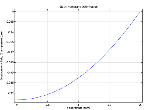
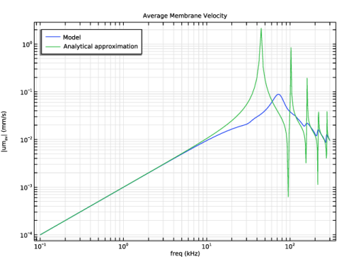
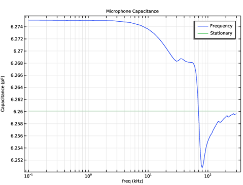
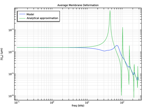
In the Settings window for 1D Plot Group, type Average Membrane Deformation in the Label text field.
3
Locate the Title section. From the Title type list, choose Label.
4
Locate the Plot Settings section.
5
Select the y-axis label checkbox. In the associated text field, type |U<sub>av</sub>| (µm).
6
Locate the Legend section. From the Position list, choose Upper left.
Global 1
1
Right-click Average Membrane Deformation and choose Global.
2
In the Settings window for Global, locate the y-Axis Data section.
3
4
In the Average Membrane Deformation toolbar, click  Plot.
5
Click the  x-Axis Log Scale button in the Graphics toolbar.
6
Click the  y-Axis Log Scale button in the Graphics toolbar.
The microphone sensitivity curve should look like Figure 3.
Finally, plot the membrane deformation and pressure distribution using a 3D revolved geometry using a 2D revolution dataset, to reproduce Figure 4.
Revolution 2D 1
1
In the Results toolbar, click  More Datasets and choose Revolution 2D.
2
In the Settings window for Revolution 2D, click to expand the Revolution Layers section.
3
In the Start angle text field, type -90.
4
In the Revolution angle text field, type 290.
Selection
In the Results toolbar, click  Attributes and choose Selection.
Membrane Deformation and Pressure
1
In the Results toolbar, click  3D Plot Group.
2
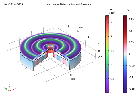
In the Settings window for 3D Plot Group, type Membrane Deformation and Pressure in the Label text field.
3
Click to expand the Title section. From the Title type list, choose Label.
4
Locate the Color Legend section. Select the Show units checkbox.
Surface 1
1
Right-click Membrane Deformation and Pressure and choose Surface.
2
In the Settings window for Surface, click Replace Expression in the upper-right corner of the Expression section. From the menu, choose Component 1 (comp1) > Membrane > Displacement > mbrn.disp - Displacement magnitude - m.
3
Locate the Coloring and Style section. From the Color table list, choose SpectrumLight.
Deformation 1
1
Right-click Surface 1 and choose Deformation.
2
In the Settings window for Deformation, click Replace Expression in the upper-right corner of the Expression section. From the menu, choose Component 1 (comp1) > Membrane > Displacement > um,vm,wm - Displacement field.
Transformation 1
1
In the Model Builder window, right-click Surface 1 and choose Transformation.
2
In the Settings window for Transformation, locate the Transformation section.
3
In the z text field, type 0.1[mm].
4
Clear the Apply to dataset edges checkbox.
Surface 2
1
In the Model Builder window, right-click Membrane Deformation and Pressure and choose Surface.
2
In the Settings window for Surface, locate the Expression section.
3
In the Expression text field, type ta.p_t.
4
Locate the Coloring and Style section. From the Color table list, choose Wave.
5
From the Scale list, choose Linear symmetric.
6
In the Membrane Deformation and Pressure toolbar, click  Plot.
The 3D plot should look like Figure 4.
As a final analysis set up a study for computing the capacitance of the microphone.
Add Study
1
In the Home toolbar, click  Add Study to open the Add Study window.
2
Go to the Add Study window.
3
Find the Physics interfaces in study subsection. In the table, clear the Solve checkbox for Thermoviscous Acoustics, Frequency Domain (ta).
4
Find the Multiphysics couplings in study subsection. In the table, clear the Solve checkbox for Thermoviscous Acoustic–Structure Boundary 1 (tsb1).
5
Find the Studies subsection. In the Select Study tree, select General Studies > Stationary.
6
Click the Add Study button in the window toolbar.
7
In the Home toolbar, click  Add Study to close the Add Study window.
Study 2 - Capacitance
1
In the Settings window for Study, type Study 2 - Capacitance in the Label text field.
2
Locate the Study Settings section. Clear the Generate default plots checkbox.
Step 1: Stationary
1
In the Model Builder window, under Study 2 - Capacitance click Step 1: Stationary.
2
In the Settings window for Stationary, locate the Physics and Variables Selection section.
3
Select the Modify model configuration for study step checkbox.
4
In the tree, select Component 1 (comp1) > Electrical Circuit (cir) > Resistor 2 (R2) and Component 1 (comp1) > Electrical Circuit (cir) > Voltage Source 2 - AC: linper(1) (V2).
5
Click  Disable.
Step 2: Frequency-Domain Perturbation
1
In the Study toolbar, click  More Study Steps and choose Frequency Domain > Frequency-Domain Perturbation.
2
In the Settings window for Frequency-Domain Perturbation, locate the Study Settings section.
3
From the Frequency unit list, choose kHz.
4
In the Frequencies text field, type {0.1 range(2.5,2.5,300)}.
Disable the incident pressure load on the membrane. For the capacitance analysis the membrane is driven by a voltage source.
5
Locate the Physics and Variables Selection section. Select the Modify model configuration for study step checkbox.
6
In the tree, select Component 1 (comp1) > Membrane (mbrn), Controls spatial frame > Face Load 1 - Incident Pressure.
7
Click  Disable.
8
In the Study toolbar, click  Compute.
Results
Microphone Capacitance
1
In the Results toolbar, click  1D Plot Group.
2
In the Settings window for 1D Plot Group, type Microphone Capacitance in the Label text field.
3
Locate the Title section. From the Title type list, choose Label.
4
Locate the Plot Settings section.
5
Select the y-axis label checkbox. In the associated text field, type Capacitance (pF).
6
Locate the Axis section. Select the x-axis log scale checkbox.
Global 1
1
Right-click Microphone Capacitance and choose Global.
2
In the Settings window for Global, locate the Data section.
3
From the Dataset list, choose Study 2 - Capacitance/Solution 3 (sol3).
4
Locate the y-Axis Data section. In the table, enter the following settings:
5
In the Microphone Capacitance toolbar, click  Plot.