|
|
|
|
•
|
A Thermoviscous Acoustics, Frequency Domain interface, which is the detailed acoustic physics interface that explicitly includes and solves for thermal and viscous loss effects.
|
|
•
|
An Electrostatics interface captures the changes in the electric field and electrostatic forces.
|
|
•
|
A Membrane interface, for setting up a pretensioned physics for the diaphragm.
|
|
•
|
A Moving Mesh feature, for modeling the static deformation of the membrane and computational domain when prepolarizing the microphone. The Moving Mesh is also solved for in the frequency domain. This ensures the coupling between the membrane movement and the electrostatic physics. The mesh movement solved for in the frequency domain (perturbation) step represents a linear (small signal) effect on top of the initial DC deformation.
|
|
•
|
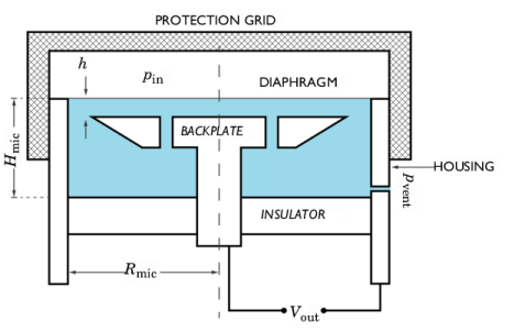
In this model it is assumed that the charge Q0 is constant. This is not fully correct. Electric interaction between the microphone and the external circuit of the preamplifier induces small changes in the surface charge. A constant charge corresponds to charging the microphone through an infinitely large resistor. This means that only the acoustic cutoff is modeled at the low frequencies and not the usual combined electric and acoustic cutoff. An example of how to include a small external electrical circuit can be seen in the Axisymmetric Condenser Microphone tutorial model.
|
|
•
|
The incident pressure field pin is constant across the membrane. This is true for normal incidence. For oblique incidence, the diaphragm diameter 2Rmic becomes comparable to half a wavelength λ/2 for f = 20 kHz.
|
|
•
|
|
•
|


|
5 μm
|
||
|
1
|
|
2
|
In the Select Physics tree, select Acoustics > Thermoviscous Acoustics > Thermoviscous Acoustics, Frequency Domain (ta).
|
|
3
|
Click Add.
|
|
4
|
|
5
|
Click Add.
|
|
6
|
|
7
|
In the Displacement field components table, enter the following settings:
|
|
8
|
|
9
|
Click Add.
|
|
10
|
Click
|
|
1
|
|
2
|
|
3
|
Click
|
|
4
|
Browse to the model’s Application Libraries folder and double-click the file bk_4134_microphone_parameters.txt.
|
|
1
|
|
2
|
|
3
|
Click
|
|
4
|
Browse to the model’s Application Libraries folder and double-click the file bk_4134_microphone.mphbin.
|
|
5
|
Click
|
|
1
|
|
2
|
|
1
|
|
2
|
|
3
|
|
4
|
Click
|
|
5
|
Browse to the model’s Application Libraries folder and double-click the file bk_4134_microphone_sensitivity_data.txt.
|
|
6
|
Click
|
|
7
|
Locate the Data Column Settings section. In the table, enter the following settings:
|
|
8
|
|
10
|
|
12
|
|
1
|
|
2
|
|
3
|
|
5
|
|
1
|
|
2
|
|
3
|
|
4
|
|
6
|
|
1
|
|
2
|
|
3
|
|
1
|
|
2
|
|
3
|
|
1
|
|
2
|
|
3
|
|
1
|
|
2
|
Go to the Add Material window.
|
|
3
|
|
4
|
Click the Add to Component button in the window toolbar.
|
|
1
|
In the Model Builder window, under Component 1 (comp1) right-click Materials and choose Blank Material.
|
|
2
|
|
3
|
Locate the Geometric Entity Selection section. From the Geometric entity level list, choose Boundary.
|
|
4
|
|
5
|
Locate the Material Contents section. In the table, enter the following settings:
|
|
6
|
|
1
|
|
2
|
|
3
|
|
1
|
|
2
|
|
3
|
|
4
|
Locate the Pressure section. In the pbnd text field, type linper(pvent_e*exp(-ta.iomega*Hmic/343[m/s])).
|
|
1
|
|
2
|
|
3
|
|
4
|
|
1
|
|
2
|
|
3
|
|
1
|
In the Model Builder window, under Component 1 (comp1) > Membrane (mbrn) click Thickness and Offset 1.
|
|
2
|
|
3
|
|
1
|
|
2
|
|
3
|
|
1
|
|
1
|
|
1
|
|
2
|
|
3
|
|
4
|
|
5
|
|
1
|
|
1
|
|
2
|
|
3
|
|
1
|
|
2
|
|
3
|
|
4
|
|
1
|
|
2
|
|
3
|
|
1
|
|
2
|
|
3
|
|
1
|
|
1
|
|
2
|
|
3
|
|
1
|
In the Physics toolbar, click
|
|
2
|
In the Settings window for Thermoviscous Acoustic–Structure Boundary, locate the Boundary Selection section.
|
|
3
|
|
1
|
In the Physics toolbar, click
|
|
1
|
|
1
|
|
1
|
|
2
|
|
1
|
|
2
|
|
3
|
Click the Custom button.
|
|
4
|
Locate the Element Size Parameters section.
|
|
5
|
|
1
|
|
2
|
|
3
|
|
5
|
|
6
|
Locate the Element Size Parameters section.
|
|
7
|
|
8
|
Click
|
|
9
|
|
1
|
|
2
|
|
3
|
|
1
|
|
2
|
|
3
|
Click
|
|
5
|
|
1
|
|
2
|
|
3
|
Click
|
|
5
|
|
6
|
|
7
|
|
8
|
|
9
|
Click
|
|
1
|
|
2
|
|
3
|
Click the Custom button.
|
|
4
|
Locate the Element Size Parameters section.
|
|
5
|
|
6
|
Click
|
|
1
|
|
2
|
|
3
|
Clear the Smooth transition to interior mesh checkbox.
|
|
1
|
|
3
|
|
4
|
|
5
|
|
6
|
|
7
|
Click
|
|
1
|
|
2
|
Go to the Add Study window.
|
|
3
|
Find the Physics interfaces in study subsection. In the table, clear the Solve checkbox for Thermoviscous Acoustics, Frequency Domain (ta).
|
|
4
|
|
5
|
Click the Add Study button in the window toolbar.
|
|
6
|
|
1
|
|
2
|
|
1
|
In the Study toolbar, click
|
|
2
|
|
3
|
|
4
|
Locate the Physics and Variables Selection section. Select the Modify model configuration for study step checkbox.
|
|
5
|
In the tree, select Component 1 (comp1) > Thermoviscous Acoustics, Frequency Domain (ta) > Pressure (Adiabatic) 2.
|
|
6
|
Right-click and choose Disable.
|
|
1
|
|
2
|
|
3
|
In the Model Builder window, expand the Study 1 - Vent Exposed > Solver Configurations > Solution 1 (sol1) > Stationary Solver 2 node, then click Suggested Direct Solver (tsb1_emfb1).
|
|
4
|
|
5
|
|
6
|
In the Model Builder window, under Study 1 - Vent Exposed > Solver Configurations > Solution 1 (sol1) > Stationary Solver 2 right-click Suggested Iterative Solver (GMRES with Direct Precond.) (tsb1_emfb1) and choose Enable.
|
|
7
|
|
1
|
|
2
|
Go to the Add Study window.
|
|
3
|
Find the Physics interfaces in study subsection. In the table, clear the Solve checkbox for Thermoviscous Acoustics, Frequency Domain (ta).
|
|
4
|
|
5
|
Click the Add Study button in the window toolbar.
|
|
6
|
|
1
|
|
2
|
|
1
|
In the Study toolbar, click
|
|
2
|
|
3
|
|
4
|
Locate the Physics and Variables Selection section. Select the Modify model configuration for study step checkbox.
|
|
5
|
In the tree, select Component 1 (comp1) > Thermoviscous Acoustics, Frequency Domain (ta) > Pressure (Adiabatic) 1.
|
|
6
|
Right-click and choose Disable.
|
|
1
|
|
2
|
|
3
|
In the Model Builder window, expand the Study 2 - Vent Unexposed > Solver Configurations > Solution 3 (sol3) > Stationary Solver 2 node, then click Suggested Direct Solver (tsb1_emfb1).
|
|
4
|
|
5
|
|
6
|
In the Model Builder window, under Study 2 - Vent Unexposed > Solver Configurations > Solution 3 (sol3) > Stationary Solver 2 right-click Suggested Iterative Solver (GMRES with Direct Precond.) (tsb1_emfb1) and choose Enable.
|
|
7
|
|
•
|
|
1
|
In the Model Builder window, expand the Results > Datasets node, then click Study 1 - Vent Exposed/Solution 1 (sol1).
|
|
2
|
|
3
|
|
1
|
|
2
|
|
3
|
|
4
|
|
5
|
|
6
|
|
1
|
|
2
|
In the Settings window for Global Evaluation, click Replace Expression in the upper-right corner of the Expressions section. From the menu, choose Component 1 (comp1) > Electrostatics > Terminals > es.V0_1 - Terminal voltage - V.
|
|
3
|
|
4
|
Click
|
|
1
|
|
2
|
|
3
|
|
4
|
|
1
|
|
2
|
|
3
|
|
4
|
|
5
|
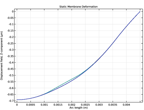
Click Replace Expression in the upper-right corner of the Expression section. From the menu, choose Component 1 (comp1) > Membrane > Displacement > mbrn.disp - Displacement magnitude - m.
|
|
6
|
|
1
|
|
2
|
|
3
|
|
1
|
|
2
|
|
3
|
|
4
|
|
1
|
|
2
|
|
3
|
|
1
|
|
2
|
|
3
|
|
4
|
|
5
|
|
6
|
|
1
|
|
2
|
|
3
|
|
1
|
|
2
|
|
3
|
|
4
|
|
1
|
|
2
|
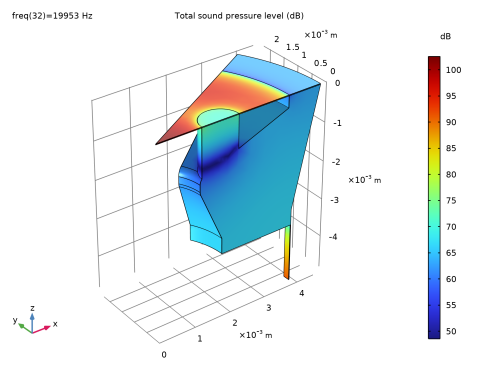
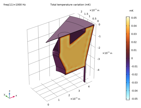
In the Settings window for 3D Plot Group, type Acoustic Temperature Variation in the Label text field.
|
|
3
|
|
4
|
|
1
|
|
2
|
|
3
|
|
4
|
|
5
|
|
6
|
|
7
|
|
1
|
|
2
|
In the Settings window for 3D Plot Group, type Electric Potential (stationary) in the Label text field.
|
|
3
|
|
4
|
|
1
|
|
2
|
|
3
|
|
4
|
|
5
|
|
6
|
|
7
|
|
1
|
|
2
|
|
3
|
|
4
|
Locate the Plot Settings section.
|
|
5
|
|
6
|
|
7
|
|
1
|
|
2
|
|
4
|
|
5
|
|
1
|
|
2
|
|
3
|
|
4
|
Locate the y-Axis Data section. In the table, enter the following settings:
|
|
5
|
|
1
|
|
2
|
|
3
|
|
1
|
|
2
|
|
3
|
|
4
|
|
6
|
|
1
|
|
2
|
|
3
|
|
4
|
|
6
|
|
7
|
|
1
|
|
2
|
|
1
|
|
2
|
|
3
|
|
1
|
|
2
|
|
3
|
|
4
|
|
1
|
|
2
|
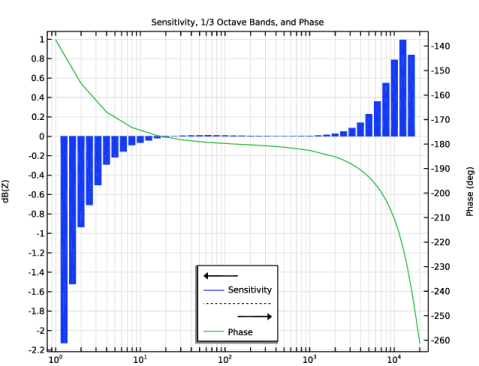
In the Settings window for 1D Plot Group, type Sensitivity, 1/3 Octave Bands, and Phase in the Label text field.
|
|
3
|
|
1
|
|
2
|
|
3
|
|
4
|
|
5
|
|
6
|
|
7
|
|
8
|
|
9
|
|
10
|
|
1
|
|
3
|
Select the Unwrap phase checkbox.
|
|
1
|
|
2
|
|
3
|
Select the Two y-axes checkbox.
|
|
4
|
|
5
|
|
6
|
|
1
|
|
2
|
|
3
|
|
1
|
|
2
|
|
3
|
|
4
|
|
1
|
|
2
|
|
3
|
Click
|
|
4
|
Browse to the model’s Application Libraries folder and double-click the file bk_4134_microphone_variables.txt.
|
|
1
|
|
2
|
|
3
|
|
4
|
|
5
|
Locate the Plot Settings section.
|
|
6
|
|
7
|
|
8
|
|
9
|
Select the y-axis log scale checkbox.
|
|
10
|
|
1
|
|
2
|
|
4
|
|
1
|
|
2
|
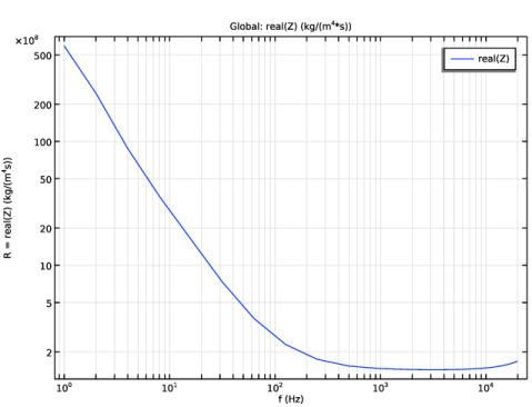
In the Settings window for 1D Plot Group, type Equivalent Acoustic Resistance in the Label text field.
|
|
3
|
|
4
|
Locate the Plot Settings section.
|
|
5
|
|
6
|
Select the y-axis label checkbox. In the associated text field, type R = real(Z) (kg/(m<sup>4</sup>s)).
|
|
7
|
|
8
|
Select the y-axis log scale checkbox.
|
|
1
|
|
2
|
|
1
|
|
2
|
|
4
|
Click to expand the Coloring and Style section. Find the Line style subsection. From the Line list, choose None.
|
|
5
|
|
6
|
|
1
|
|
2
|
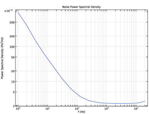
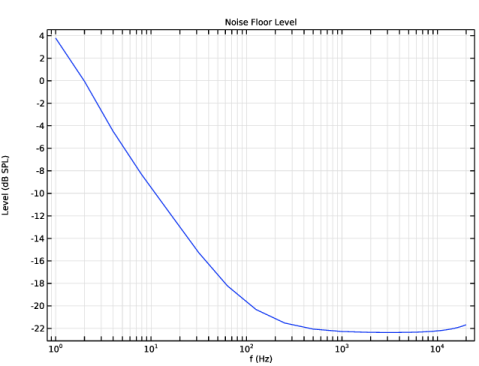
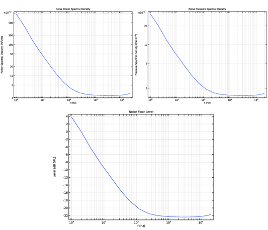
In the Settings window for 1D Plot Group, type Noise Power Spectral Density in the Label text field.
|
|
3
|
|
4
|
|
5
|
Locate the Plot Settings section.
|
|
6
|
|
7
|
Select the y-axis label checkbox. In the associated text field, type Power Spectral Density (Pa<sup>2</sup>/Hz).
|
|
8
|
|
9
|
Select the y-axis log scale checkbox.
|
|
10
|
|
1
|
|
2
|
|
4
|
|
1
|
|
2
|
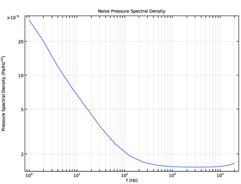
In the Settings window for 1D Plot Group, type Noise Pressure Spectral Density in the Label text field.
|
|
3
|
|
4
|
|
5
|
Locate the Plot Settings section.
|
|
6
|
|
7
|
Select the y-axis label checkbox. In the associated text field, type Pressure Spectral Density (Pa/Hz<sup>1/2</sup>).
|
|
8
|
|
9
|
Select the y-axis log scale checkbox.
|
|
10
|
|
1
|
|
2
|
|
4
|
|
1
|
|
2
|
|
3
|
|
4
|
|
5
|
Locate the Plot Settings section.
|
|
6
|
|
7
|
|
8
|
|
9
|
|
1
|
|
2
|
|
4
|
|
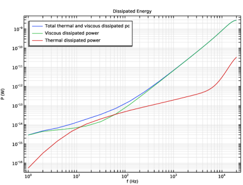
1
|
In the Model Builder window, under Results, Ctrl-click to select Dissipated Energy, Equivalent Acoustic Resistance, Noise Power Spectral Density, Noise Pressure Spectral Density, and Noise Floor Level.
|
|
2
|
Right-click and choose Group.
|