



PDF

Baffled Piston Radiation
Introduction
An axisymmetric model of a rigid piston in an infinite baffle is used to exemplify the Acoustics Module’s Exterior Field Calculation feature. The radiation results obtained with COMSOL Multiphysics are compared with analytical results for the on-axis radiation pattern (as a function of distance), the spatial far-field response, and the total radiated power. The transition from near field to far field is smooth and continuous.
Model Definition
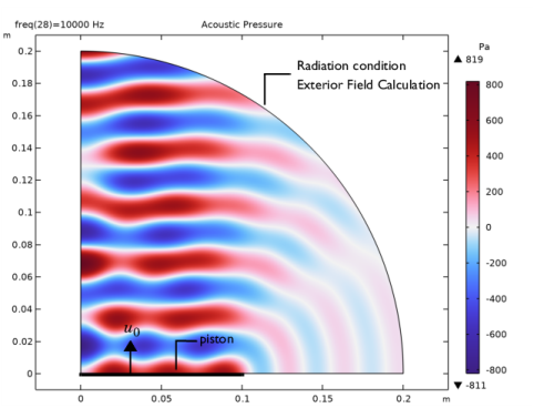
The model consists of a 2D axisymmetric piston recessed in a rigid baffle and vibrating in air. The piston radius is = 0.1 m. It will be assumed to move at a constant velocity of u0 = 1 m/s
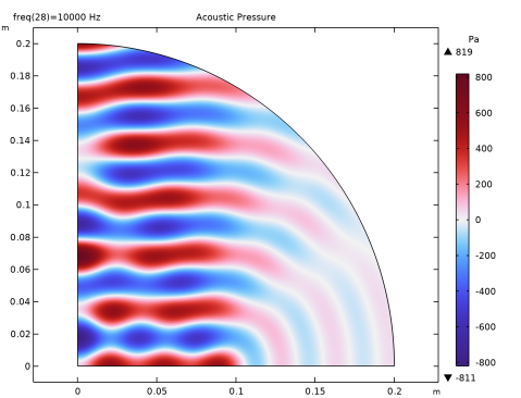
Figure 1: Geometry of the piston in an infinite baffle model. The colors represent the acoustic pressure in the air surrounding the piston at f = 10 kHz.
The piston will be excited by a range of frequencies going from 10 Hz to 20 kHz. The model parameters are given in Table 1.
As described in Jacobsen and others (Ref. 2), theoretically, the piston can be modeled as a group of uncorrelated monopoles. Supposing linear superposition, the pressure radiated by the piston can be calculated at any point of interest as an integration of the power radiated by a monopole over the surface of the piston:
(1)
Here, ω is the angular frequency, ρ the density, k the wave number, S the surface of the piston, and x the distance between the point of interest and the running position on the piston. This is a special case of the Rayleigh integral.
The Exterior Field Calculation feature uses the full Kirchhoff–Helmholtz integral, which is valid at any point outside the computational domain. When applied to a flat surface, it reduces to the Rayleigh integral.
Far Field
As explained in Jacobsen and others (Ref. 2), the pressure in the far-field approximation can be written using Bessel functions J0(z) and J1(z), giving
(2)
where θ is the polar angle and r the distance from the center of the piston.
Near Field
In the near-field approximation, it is not possible to derive an analytical expression for the pressure. However, the force exerted on the piston (or the radiation impedance) can be calculated and is presented in Ref. 1. In the analytical force expression, there is a need to introduce Bessel and Struve functions. The Struve function can be approximated by (see Ref. 3)
(3)
(The Struve function is also often denoted H1.) The force on the piston can then be written as
(4)
which by division with the velocity and area gives the radiation impedance. The analytical expressions given above are implemented using variable definitions and integration coupling operators.
Results and Discussion
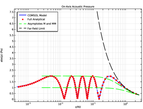
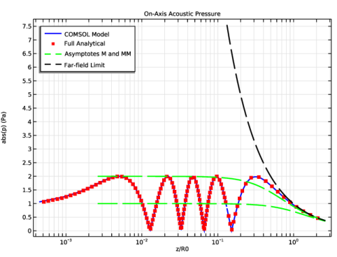
Figure 2 shows the computed COMSOL on-axis pressure as well as the analytical results, the asymptotes M and MM, and the far-field limit. First, it is noticeable that the COMSOL and analytical results are really similar.
Figure 2: On-axis pressure as a function of z/R0 (logarithmic axis).
From a theoretical aspect, the pressure zeros in Figure 2 can be explained with the so-called monopole model. All the monopoles will interfere destructively and cancel out, resulting in the pressure being zero. According to Blackstock (Ref. 1), the number of zeros, n, depends on the value of a/λ. If this ratio is an integer, then n = a/λ and the first zero is at the piston itself. If it is not an integer, then (where means “the integer part of”) and the first zero happens in front of the piston.

The asymptotes are also worth noticing. There is good agreement between the COMSOL model and the far-field limit. The asymptotes M and MM represent the following functions (see Ref. 1):
(5)
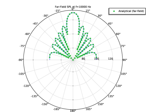
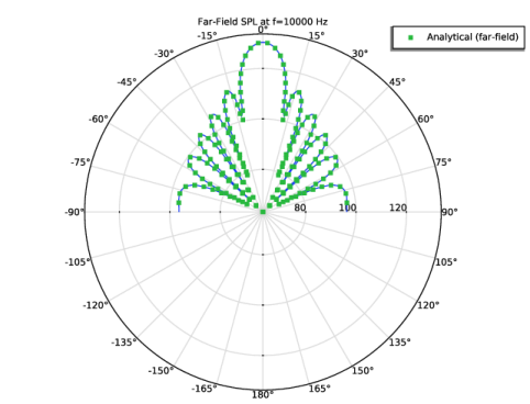
Figure 3: Far-field radiation pattern at f = 10 kHz.
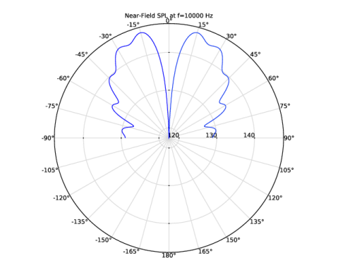
In Figure 3, the radiation pattern of the actual far field, further away than the Rayleigh distance R0, is plotted at f = 10 kHz. As expected, it shows strong directivity at this frequency; there is a clear focus in the on-axial direction. However, there are still some sidelobes present in other directions. It should be noted that at low frequencies, the piston can behave as a strictly omnidirectional source, because, according to the representation by monopoles, they would all move in phase. Figure 3 also shows good agreement between the simulated and analytical solutions.
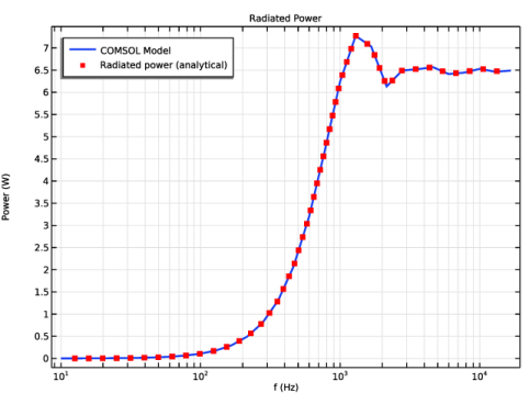
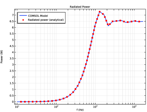
In Figure 4, the analytical total radiated power is compared with the result of the COMSOL simulation. They have really similar results from low to high frequencies. It goes from no radiated power to a maximum for the critical frequency before decreasing again to reach a steady state.
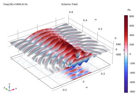
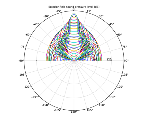
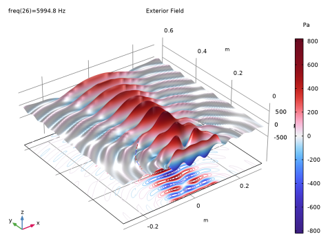
Finally, Figure 5 represents the acoustic field created by the piston, both in the computational domain and exterior to the domain. This is achieved using the Exterior Field Calculation feature combined with visualization in a Grid 2D dataset. The feature allows the calculation and the visualization of the pressure field outside the computational domain at any distance including amplitude and phase.
Figure 4: Total radiated power as a function of frequency.
Figure 5: Pressure field near the piston surface.
References
1. D. Blackstock, “Fundamentals of physical acoustics,” Wiley-interscience, 2000.
2. F. Jacobsen, T. Poulsen, J.H. Rindel, A.C. Gade, and M. Ohlrich, Fundamentals of Acoustics and Noise Control, Technical University of Denmark, Department of Electrical Engineering, 2008.
3. R.M. Aerts and A.J.E.M. Janssen, “Efficient approximation of the Struve functions Hn occurring in the calculation of sound radiation quantities,” J. Acoust. Soc. Am., vol. 140, pp. 4154–4160, 2016.
Application Library path: Acoustics_Module/Verification_Examples/baffled_piston_radiation
Modeling Instructions
From the File menu, choose New.
New
In the New window, click  Model Wizard.
Model Wizard
1
In the Model Wizard window, click  2D Axisymmetric.
2
In the Select Physics tree, select Acoustics > Pressure Acoustics > Pressure Acoustics, Frequency Domain (acpr).
3
Click Add.
4
Click  Study.
5
In the Select Study tree, select General Studies > Frequency Domain.
6
Global Definitions
Parameters 1
1
In the Model Builder window, under Global Definitions click Parameters 1.
2
In the Settings window for Parameters, locate the Parameters section.
3
Click  Load from File.
4
Geometry 1
Circle 1 (c1)
1
In the Geometry toolbar, click  Circle.
2
In the Settings window for Circle, locate the Size and Shape section.
3
In the Radius text field, type Rmodel.
4
In the Sector angle text field, type 90.
Point 1 (pt1)
1
In the Geometry toolbar, click  Point.
2
In the Settings window for Point, locate the Point section.
3
In the r text field, type a.
4
Click  Build All Objects.
Definitions
Variables: Analytical Pressure Field
1
In the Definitions toolbar, click  Local Variables.
2
In the Settings window for Variables, type Variables: Analytical Pressure Field in the Label text field.
3
Locate the Variables section. Click  Load from File.
4
Variables: Surface Impedance and Power
1
In the Definitions toolbar, click  Local Variables.
2
In the Settings window for Variables, type Variables: Surface Impedance and Power in the Label text field.
3
Locate the Variables section. Click  Load from File.
4
Integration 1 (intop1)
1
In the Definitions toolbar, click  Nonlocal Couplings and choose Integration.
2
In the Settings window for Integration, type intop_pt in the Operator name text field.
3
Locate the Source Selection section. From the Geometric entity level list, choose Point.
4
Click  Paste Selection.
5
In the Paste Selection dialog, type 1 in the Selection text field.
6
7
In the Settings window for Integration, locate the Advanced section.
8
Clear the Compute integral in revolved geometry checkbox.
Integration 2 (intop2)
1
In the Definitions toolbar, click  Nonlocal Couplings and choose Integration.
2
In the Settings window for Integration, type intop_out in the Operator name text field.
3
Locate the Source Selection section. From the Geometric entity level list, choose Boundary.
4
Click  Paste Selection.
5
In the Paste Selection dialog, type 4 in the Selection text field.
6
Add Material
1
In the Materials toolbar, click  Add Material to open the Add Material window.
2
Go to the Add Material window.
3
In the tree, select Built-in > Air.
4
Click the Add to Component button in the window toolbar.
5
In the Materials toolbar, click  Add Material to close the Add Material window.
Pressure Acoustics, Frequency Domain (acpr)
Pressure Acoustics 1
1
In the Settings window for Pressure Acoustics, locate the Pressure Acoustics Model section.
2
From the Fluid model list, choose Atmosphere attenuation.
Normal Velocity 1
1
In the Physics toolbar, click  Boundaries and choose Normal Velocity.
2
In the Settings window for Normal Velocity, locate the Boundary Selection section.
3
Click  Paste Selection.
4
In the Paste Selection dialog, type 2 in the Selection text field.
5
6
In the Settings window for Normal Velocity, locate the Normal Velocity section.
7
In the vn text field, type u0.
Spherical Wave Radiation 1
1
In the Physics toolbar, click  Boundaries and choose Spherical Wave Radiation.
2
In the Settings window for Spherical Wave Radiation, locate the Boundary Selection section.
3
Click  Paste Selection.
4
In the Paste Selection dialog, type 4 in the Selection text field.
5
Exterior Field Calculation 1
1
In the Physics toolbar, click  Boundaries and choose Exterior Field Calculation.
2
In the Settings window for Exterior Field Calculation, locate the Boundary Selection section.
3
Click  Paste Selection.
4
In the Paste Selection dialog, type 4 in the Selection text field.
5
6
In the Settings window for Exterior Field Calculation, locate the Exterior Field Calculation section.
7
From the Condition in the z = z0 plane list, choose Symmetric/Infinite sound hard boundary.
Study 1
1
In the Model Builder window, click Study 1.
2
In the Settings window for Study, locate the Study Settings section.
3
Clear the Generate default plots checkbox.
Step 1: Frequency Domain
1
In the Model Builder window, under Study 1 click Step 1: Frequency Domain.
2
In the Settings window for Frequency Domain, locate the Study Settings section.
3
Click  Range.
4
In the Range dialog, choose Logarithmic from the Entry method list.
5
In the Start text field, type 10.
6
In the Stop text field, type 20000.
7
In the Steps per decade text field, type 9.
8
Click Replace.
9
In the Settings window for Frequency Domain, locate the Study Settings section.
10
From the Reuse solution from previous step list, choose Yes.
Solution 1 (sol1)
In the Study toolbar, click  Show Default Solver.
Mesh 1
In the Model Builder window, under Component 1 (comp1) right-click Mesh 1 and choose Build All.
Study 1
In the Study toolbar, click  Compute.
Results
In the Model Builder window, expand the Results node.
Parametric Curve 2D 1
1
In the Model Builder window, expand the Results > Datasets node.
2
Right-click Results > Datasets and choose More 2D Datasets > Parametric Curve 2D.
3
In the Settings window for Parametric Curve 2D, locate the Parameter section.
4
In the Maximum text field, type pi/2.
5
Locate the Expressions section. In the r text field, type 1.3*a*cos(s).
6
In the z text field, type 1.3*a*sin(s).
Parametric Curve 2D 2
1
In the Results toolbar, click  More Datasets and choose Parametric Curve 2D.
2
In the Settings window for Parametric Curve 2D, locate the Expressions section.
3
In the z text field, type 1.01*Rmodel*(1-s)+Rfar*s.
4
Select the Only evaluate globally defined expressions checkbox.
Parametric Curve 2D 3
1
In the Results toolbar, click  More Datasets and choose Parametric Curve 2D.
2
In the Settings window for Parametric Curve 2D, locate the Expressions section.
3
Select the Only evaluate globally defined expressions checkbox.
Revolution 2D 1
In the Results toolbar, click  More Datasets and choose Revolution 2D.
Parametric Curve 2D 3
1
In the Model Builder window, click Parametric Curve 2D 3.
2
In the Settings window for Parametric Curve 2D, locate the Expressions section.
3
In the z text field, type Rfar*s.
Revolution 2D 1
1
In the Model Builder window, click Revolution 2D 1.
2
In the Settings window for Revolution 2D, click to expand the Revolution Layers section.
3
In the Start angle text field, type -50.
4
In the Revolution angle text field, type 230.
Grid 2D 1
1
In the Results toolbar, click  More Datasets and choose Grid > Grid 2D.
2
In the Settings window for Grid 2D, locate the Parameter Bounds section.
3
Find the First parameter subsection. In the Name text field, type r.
4
In the Minimum text field, type -1.5*Rmodel.
5
In the Maximum text field, type 1.5*Rmodel.
6
Find the Second parameter subsection. In the Name text field, type z.
7
In the Maximum text field, type 3*Rmodel.
Mirror 2D 1
1
In the Results toolbar, click  More Datasets and choose Mirror 2D.
2
In the Model Builder window, click Results.
3
In the Settings window for Results, locate the Save Data in the Model section.
4
From the Save plot data list, choose On.
Acoustic Pressure
1
In the Results toolbar, click  2D Plot Group.
2
In the Settings window for 2D Plot Group, type Acoustic Pressure in the Label text field.
3
Locate the Data section. From the Parameter value (freq (Hz)) list, choose 10000.
4
Click to expand the Title section. From the Title type list, choose Label.
5
Locate the Color Legend section. Select the Show maximum and minimum values checkbox.
6
Select the Show units checkbox.
Surface 1
1
In the Acoustic Pressure toolbar, click  Surface.
2
In the Settings window for Surface, locate the Coloring and Style section.
3
From the Color table list, choose Wave.
4
In the Acoustic Pressure toolbar, click  Plot.
On-Axis Acoustic Pressure
1
In the Results toolbar, click  1D Plot Group.
2
In the Settings window for 1D Plot Group, type On-Axis Acoustic Pressure in the Label text field.
3
Locate the Data section. From the Parameter selection (freq) list, choose Last.
4
Click to expand the Title section. From the Title type list, choose Label.
5
Locate the Plot Settings section.
6
Select the x-axis label checkbox. In the associated text field, type z/R0.
7
Select the y-axis label checkbox. In the associated text field, type abs(p) (Pa).
8
Locate the Axis section. Select the x-axis log scale checkbox.
9
Locate the Legend section. From the Position list, choose Upper left.
Line Graph 1
1
In the On-Axis Acoustic Pressure toolbar, click  Line Graph.
2
In the Settings window for Line Graph, locate the Selection section.
3
Click  Paste Selection.
4
In the Paste Selection dialog, type 1 in the Selection text field.
5
6
In the Settings window for Line Graph, locate the y-Axis Data section.
7
In the Expression text field, type abs(p/p0).
8
Locate the x-Axis Data section. From the Parameter list, choose Expression.
9
In the Expression text field, type z/R0.
10
Click to expand the Coloring and Style section. From the Color list, choose Blue.
11
From the Width list, choose 2.
12
Click to expand the Legends section. Select the Show legends checkbox.
13
From the Legends list, choose Manual.
14
On-Axis Acoustic Pressure
In the Model Builder window, click On-Axis Acoustic Pressure.
Line Graph 2
1
In the On-Axis Acoustic Pressure toolbar, click  Line Graph.
2
In the Settings window for Line Graph, locate the Selection section.
3
Click  Paste Selection.
4
In the Paste Selection dialog, type 1 in the Selection text field.
5
6
In the Settings window for Line Graph, locate the y-Axis Data section.
7
In the Expression text field, type abs(p_axis/p0).
8
Locate the x-Axis Data section. From the Parameter list, choose Expression.
9
In the Expression text field, type z/R0.
10
Locate the Coloring and Style section. Find the Line style subsection. From the Line list, choose None.
11
From the Color list, choose Red.
12
From the Width list, choose 2.
13
Find the Line markers subsection. From the Marker list, choose Point.
14
From the Positioning list, choose Interpolated.
15
In the Number text field, type 100.
16
Locate the Legends section. Select the Show legends checkbox.
17
From the Legends list, choose Manual.
18
On-Axis Acoustic Pressure
In the Model Builder window, click On-Axis Acoustic Pressure.
Line Graph 3
1
In the On-Axis Acoustic Pressure toolbar, click  Line Graph.
2
In the Settings window for Line Graph, locate the Data section.
3
From the Dataset list, choose Parametric Curve 2D 2.
4
From the Parameter selection (freq) list, choose Last.
5
Locate the y-Axis Data section. In the Expression text field, type abs(pext(0,z)/p0).
6
Locate the x-Axis Data section. From the Parameter list, choose Expression.
7
In the Expression text field, type z/R0.
8
Locate the Coloring and Style section. From the Color list, choose Blue.
9
From the Width list, choose 2.
10
Locate the Legends section. From the Legends list, choose Manual.
11
On-Axis Acoustic Pressure
In the Model Builder window, click On-Axis Acoustic Pressure.
Line Graph 4
1
In the On-Axis Acoustic Pressure toolbar, click  Line Graph.
2
In the Settings window for Line Graph, locate the Data section.
3
From the Dataset list, choose Parametric Curve 2D 2.
4
From the Parameter selection (freq) list, choose Last.
5
Locate the y-Axis Data section. In the Expression text field, type abs(p_axis_ff/p0).
6
Locate the x-Axis Data section. From the Parameter list, choose Expression.
7
In the Expression text field, type z/R0.
8
Locate the Coloring and Style section. Find the Line style subsection. From the Line list, choose None.
9
From the Color list, choose Red.
10
From the Width list, choose 2.
11
Find the Line markers subsection. From the Marker list, choose Point.
12
From the Positioning list, choose Interpolated.
13
In the Number text field, type 20.
On-Axis Acoustic Pressure
In the Model Builder window, click On-Axis Acoustic Pressure.
Line Graph 5
1
In the On-Axis Acoustic Pressure toolbar, click  Line Graph.
2
In the Settings window for Line Graph, locate the Data section.
3
From the Dataset list, choose Parametric Curve 2D 3.
4
From the Parameter selection (freq) list, choose Last.
5
Locate the y-Axis Data section. In the Expression text field, type 2/sqrt(1+(2*z/R0)^2).
6
Locate the x-Axis Data section. From the Parameter list, choose Expression.
7
In the Expression text field, type z/R0.
8
Locate the Coloring and Style section. Find the Line style subsection. From the Line list, choose Dashed.
9
From the Color list, choose Green.
10
From the Width list, choose 2.
11
Locate the Legends section. Select the Show legends checkbox.
12
From the Legends list, choose Manual.
13
On-Axis Acoustic Pressure
In the Model Builder window, click On-Axis Acoustic Pressure.
Line Graph 6
1
In the On-Axis Acoustic Pressure toolbar, click  Line Graph.
2
In the Settings window for Line Graph, locate the Data section.
3
From the Dataset list, choose Parametric Curve 2D 3.
4
From the Parameter selection (freq) list, choose Last.
5
Locate the y-Axis Data section. In the Expression text field, type 1/sqrt(1+(z/R0)^2).
6
Locate the x-Axis Data section. From the Parameter list, choose Expression.
7
In the Expression text field, type z/R0.
8
Locate the Coloring and Style section. Find the Line style subsection. From the Line list, choose Dashed.
9
From the Color list, choose Green.
10
From the Width list, choose 2.
On-Axis Acoustic Pressure
In the Model Builder window, click On-Axis Acoustic Pressure.
Line Graph 7
1
In the On-Axis Acoustic Pressure toolbar, click  Line Graph.
2
In the Settings window for Line Graph, locate the Data section.
3
From the Dataset list, choose Parametric Curve 2D 2.
4
From the Parameter selection (freq) list, choose Last.
5
Locate the y-Axis Data section. In the Expression text field, type abs(i*R0/z*exp(-i*k*z)).
6
Locate the x-Axis Data section. From the Parameter list, choose Expression.
7
In the Expression text field, type z/R0.
8
Locate the Coloring and Style section. Find the Line style subsection. From the Line list, choose Dashed.
9
From the Color list, choose Black.
10
From the Width list, choose 2.
11
Locate the Legends section. Select the Show legends checkbox.
12
From the Legends list, choose Manual.
13
14
In the On-Axis Acoustic Pressure toolbar, click  Plot.
The on-axis pressure should look like the one in the figure below.
Near Field r=1.3a
1
In the Home toolbar, click  Add Plot Group and choose Polar Plot Group.
2
In the Settings window for Polar Plot Group, type Near Field r=1.3a in the Label text field.
3
Locate the Data section. From the Dataset list, choose Parametric Curve 2D 1.
4
From the Parameter selection (freq) list, choose From list.
5
In the Parameter values (freq (Hz)) list box, select 10000.
6
Click to expand the Title section. From the Title type list, choose Manual.
7
In the Title text area, type Near-Field SPL at f=eval(freq) Hz.
8
Locate the Axis section. Select the Symmetric angle range checkbox.
9
From the Zero angle list, choose Up.
10
From the Rotation direction list, choose Clockwise.
Line Graph 1
1
In the Near Field r=1.3a toolbar, click  Line Graph.
2
In the Settings window for Line Graph, locate the r-Axis Data section.
3
In the Expression text field, type acpr.Lp.
4
Locate the θ Angle Data section. From the Parameter list, choose Expression.
5
In the Expression text field, type theta.
6
In the Unit field, type 1.
Near Field r=1.3a
In the Model Builder window, click Near Field r=1.3a.
Line Graph 2
1
In the Near Field r=1.3a toolbar, click  Line Graph.
2
In the Settings window for Line Graph, locate the r-Axis Data section.
3
In the Expression text field, type acpr.Lp.
4
Locate the θ Angle Data section. From the Parameter list, choose Expression.
5
In the Expression text field, type -theta.
6
In the Unit field, type 1.
7
Click to expand the Coloring and Style section. From the Color list, choose Blue.
8
In the Near Field r=1.3a toolbar, click  Plot.
Far Field r=Rfar
1
In the Results toolbar, click  Polar Plot Group.
2
In the Settings window for Polar Plot Group, type Far Field r=Rfar in the Label text field.
3
Locate the Data section. From the Parameter selection (freq) list, choose From list.
4
In the Parameter values (freq (Hz)) list box, select 10000.
5
Locate the Title section. From the Title type list, choose Manual.
6
In the Title text area, type Far-Field SPL at f=eval(freq) Hz.
7
Locate the Axis section. Select the Symmetric angle range checkbox.
8
From the Zero angle list, choose Up.
9
From the Rotation direction list, choose Clockwise.
Radiation Pattern 1
1
In the Far Field r=Rfar toolbar, click  More Plots and choose Radiation Pattern.
2
In the Settings window for Radiation Pattern, locate the Evaluation section.
3
Find the Angles subsection. In the Number of angles text field, type 180.
4
From the Restriction list, choose Manual.
5
In the ϕ start text field, type -90.
6
In the ϕ range text field, type 180.
7
Find the Evaluation distance subsection. In the Radius text field, type Rfar.
8
In the Far Field r=Rfar toolbar, click  Plot.
Far Field r=Rfar
In the Model Builder window, click Far Field r=Rfar.
Radiation Pattern 2
1
In the Far Field r=Rfar toolbar, click  More Plots and choose Radiation Pattern.
2
In the Settings window for Radiation Pattern, locate the Expression section.
3
In the Expression text field, type 10*log10(0.5*p_ana*conj(p_ana)/(20e-6)^2).
4
Locate the Evaluation section. Find the Angles subsection. In the Number of angles text field, type 180.
5
From the Restriction list, choose Manual.
6
In the ϕ start text field, type -90.
7
In the ϕ range text field, type 180.
8
Find the Evaluation distance subsection. In the Radius text field, type Rfar.
9
Click to expand the Legends section. Select the Show legends checkbox.
10
From the Legends list, choose Manual.
11
12
Click to expand the Coloring and Style section. Find the Line style subsection. From the Line list, choose None.
13
Find the Line markers subsection. From the Marker list, choose Point.
14
From the Positioning list, choose Interpolated.
15
In the Number text field, type 180.
16
In the Far Field r=Rfar toolbar, click  Plot.
The far-field radiation pattern at f=10,000 Hz should look like the one in the figure below.
Beamwidth Polar
1
In the Results toolbar, click  Polar Plot Group.
2
In the Settings window for Polar Plot Group, type Beamwidth Polar in the Label text field.
3
Locate the Axis section. Select the Symmetric angle range checkbox.
4
From the Zero angle list, choose Up.
5
From the Rotation direction list, choose Clockwise.
Radiation Pattern 1
1
In the Beamwidth Polar toolbar, click  More Plots and choose Radiation Pattern.
2
In the Settings window for Radiation Pattern, locate the Evaluation section.
3
Find the Angles subsection. In the Number of angles text field, type 90.
4
From the Restriction list, choose Manual.
5
In the ϕ start text field, type -90.
6
In the ϕ range text field, type 180.
7
From the Compute beamwidth list, choose On.
8
In the Level down text field, type 3.
9
Find the Evaluation distance subsection. In the Radius text field, type Rfar.
10
In the Beamwidth Polar toolbar, click  Plot.
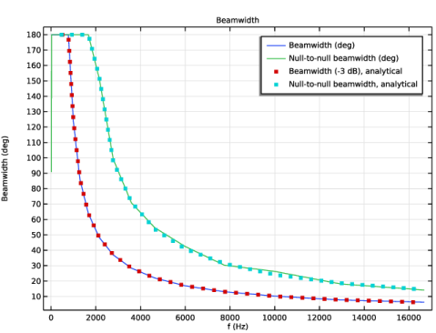
Beamwidth
1
In the Results toolbar, click  1D Plot Group.
2
In the Settings window for 1D Plot Group, type Beamwidth in the Label text field.
3
Locate the Data section. From the Dataset list, choose None.
4
Locate the Title section. From the Title type list, choose Label.
5
Locate the Plot Settings section.
6
Select the x-axis label checkbox. In the associated text field, type f (Hz).
7
Select the y-axis label checkbox. In the associated text field, type Beamwidth (deg).
Table Graph 1
1
In the Beamwidth toolbar, click  Table Graph.
2
In the Settings window for Table Graph, click to expand the Legends section.
3
Select the Show legends checkbox.
Beamwidth
In the Beamwidth toolbar, click  Global.
Global 1
1
In the Settings window for Global, locate the Data section.
2
From the Dataset list, choose Study 1/Solution 1 (sol1).
3
Locate the y-Axis Data section. In the table, enter the following settings:
4
Click to expand the Coloring and Style section. Find the Line style subsection. From the Line list, choose None.
5
Find the Line markers subsection. From the Marker list, choose Point.
6
From the Positioning list, choose Interpolated.
7
In the Number text field, type 50.
8
In the Beamwidth toolbar, click  Plot.
Radiated Power
1
In the Results toolbar, click  1D Plot Group.
2
In the Settings window for 1D Plot Group, type Radiated Power in the Label text field.
3
Locate the Title section. From the Title type list, choose Label.
4
Locate the Plot Settings section.
5
Select the x-axis label checkbox. In the associated text field, type f (Hz).
6
Select the y-axis label checkbox. In the associated text field, type Power (W).
7
Locate the Axis section. Select the x-axis log scale checkbox.
8
Locate the Legend section. From the Position list, choose Upper left.
Global 1
1
In the Radiated Power toolbar, click  Global.
2
In the Settings window for Global, locate the y-Axis Data section.
3
4
Locate the Coloring and Style section. From the Width list, choose 2.
Radiated Power
In the Radiated Power toolbar, click  Global.
Global 2
1
In the Settings window for Global, locate the y-Axis Data section.
2
3
Locate the Coloring and Style section. Find the Line style subsection. From the Line list, choose None.
4
From the Color list, choose Red.
5
From the Width list, choose 2.
6
Find the Line markers subsection. From the Marker list, choose Point.
7
From the Positioning list, choose Interpolated.
8
In the Number text field, type 50.
9
In the Radiated Power toolbar, click  Plot.
The total radiated power should look like the one in the figure below.
Exterior Field
1
In the Results toolbar, click  2D Plot Group.
2
In the Settings window for 2D Plot Group, type Exterior Field in the Label text field.
3
Locate the Data section. From the Dataset list, choose Grid 2D 1.
4
From the Parameter value (freq (Hz)) list, choose 5994.8.
5
Locate the Title section. From the Title type list, choose Label.
6
Locate the Color Legend section. Select the Show units checkbox.
Surface 1
1
In the Exterior Field toolbar, click  Surface.
2
In the Settings window for Surface, locate the Data section.
3
From the Dataset list, choose Mirror 2D 1.
4
From the Parameter value (freq (Hz)) list, choose 5994.8.
5
Locate the Coloring and Style section. From the Color table list, choose Wave.
Height Expression 1
1
In the Exterior Field toolbar, click  Height Expression.
2
In the Settings window for Height Expression, locate the Axis section.
3
Select the Scale factor checkbox. In the associated text field, type 1.E-4.
4
In the Offset text field, type 0.15.
Exterior Field
In the Model Builder window, under Results click Exterior Field.
Surface 2
1
In the Exterior Field toolbar, click  Surface.
2
In the Settings window for Surface, locate the Expression section.
3
In the Expression text field, type pext(r,z).
4
Click to expand the Inherit Style section. From the Plot list, choose Surface 1.
Filter 1
In the Exterior Field toolbar, click  Filter.
It is necessary to use a filter here for the computation of the Kirchhoff-Helmholtz integral (Exterior Field). The kernel is not numerically well defined near the source boundaries.
1
In the Settings window for Filter, locate the Element Selection section.
2
In the Logical expression for inclusion text field, type sqrt(z^2+r^2)>1.01*Rmodel.
Surface 2
In the Model Builder window, click Surface 2.
Height Expression 1
1
In the Exterior Field toolbar, click  Height Expression.
2
In the Settings window for Height Expression, locate the Axis section.
3
In the Offset text field, type 0.15.
Exterior Field
In the Model Builder window, under Results click Exterior Field.
Contour 1
1
In the Exterior Field toolbar, click  Contour.
2
In the Settings window for Contour, locate the Data section.
3
From the Dataset list, choose Mirror 2D 1.
4
From the Parameter value (freq (Hz)) list, choose 5994.8.
5
Locate the Coloring and Style section. From the Color table list, choose Wave.
6
Clear the Color legend checkbox.
Exterior Field
In the Model Builder window, click Exterior Field.
Contour 2
1
In the Exterior Field toolbar, click  Contour.
2
In the Settings window for Contour, locate the Expression section.
3
In the Expression text field, type pext(r,z).
4
Locate the Coloring and Style section. Clear the Color legend checkbox.
5
Click to expand the Inherit Style section. From the Plot list, choose Contour 1.
Filter 1
1
In the Exterior Field toolbar, click  Filter.
2
In the Settings window for Filter, locate the Element Selection section.
3
In the Logical expression for inclusion text field, type sqrt(z^2+r^2)>1.01*Rmodel.
4
In the Exterior Field toolbar, click  Plot.
The exterior field should look like the one in the figure below.
Thumbnail
1
In the Home toolbar, click  Add Plot Group and choose 3D Plot Group.
2
In the Settings window for 3D Plot Group, type Thumbnail in the Label text field.
3
Locate the Color Legend section. Select the Show units checkbox.
Surface 1
1
In the Thumbnail toolbar, click  Surface.
2
In the Settings window for Surface, locate the Expression section.
3
In the Expression text field, type acpr.Lp.
4
Locate the Coloring and Style section. From the Color table list, choose Rainbow.
5
From the Scale list, choose Linear.
6
In the Thumbnail toolbar, click  Plot.