|
|
|


|
1
|
|
2
|
In the Select Physics tree, select Acoustics > Pressure Acoustics > Pressure Acoustics, Frequency Domain (acpr).
|
|
3
|
Click Add.
|
|
4
|
Click
|
|
5
|
|
6
|
Click
|
|
1
|
|
2
|
|
3
|
Click
|
|
4
|
Browse to the model’s Application Libraries folder and double-click the file anisotropic_porous_absorber_parameters.txt.
|
|
1
|
|
2
|
|
3
|
|
4
|
|
5
|
Click to expand the Layers section. In the table, enter the following settings:
|
|
1
|
|
2
|
|
3
|
|
1
|
|
2
|
|
3
|
|
4
|
Click
|
|
5
|
Browse to the model’s Application Libraries folder and double-click the file anisotropic_porous_absorber_variables.txt.
|
|
1
|
|
2
|
|
3
|
|
5
|
|
1
|
|
2
|
|
3
|
|
5
|
|
1
|
|
2
|
|
3
|
|
5
|
|
1
|
|
3
|
|
4
|
|
5
|
|
1
|
|
2
|
Go to the Add Material window.
|
|
3
|
|
4
|
Click the Add to Component button in the window toolbar.
|
|
5
|
|
1
|
In the Model Builder window, under Component 1 (comp1) right-click Materials and choose Blank Material.
|
|
2
|
|
3
|
Click to expand the Material Properties section. In the Material properties tree, select Basic Properties > Porosity.
|
|
4
|
Click
|
|
5
|
Locate the Material Contents section. In the table, enter the following settings:
|
|
6
|
Locate the Material Properties section. In the Material properties tree, select Acoustics > Poroacoustics Model.
|
|
7
|
Click
|
|
8
|
Locate the Material Contents section. In the table, enter the following settings:
|
|
1
|
|
3
|
|
4
|
|
5
|
|
6
|
|
7
|
Select the Calculate background and scattered field intensity checkbox.
|
|
8
|
|
1
|
|
3
|
|
4
|
|
5
|
|
1
|
|
3
|
|
4
|
|
5
|
|
1
|
|
3
|
|
4
|
|
5
|
|
1
|
|
3
|
|
4
|
|
5
|
Locate the Porous Matrix Properties section. From the Porous elastic material list, choose Porous Material (mat2).
|
|
1
|
|
2
|
|
3
|
Click the Custom button.
|
|
4
|
|
5
|
|
1
|
|
2
|
|
3
|
|
5
|
|
1
|
|
3
|
|
4
|
|
5
|
|
1
|
|
2
|
|
3
|
|
1
|
|
2
|
|
3
|
Click
|
|
4
|
|
5
|
|
6
|
|
7
|
Click Add.
|
|
8
|
|
9
|
Select the Auxiliary sweep checkbox.
|
|
10
|
Click
|
|
12
|
|
1
|
|
2
|
|
1
|
|
1
|
In the Model Builder window, expand the Component 2 (comp2) > Pressure Acoustics, Frequency Domain (acpr2) node.
|
|
2
|
Right-click Component 2 (comp2) > Pressure Acoustics, Frequency Domain (acpr2) > Anisotropic Poroacoustics 1 and choose Delete.
|
|
1
|
|
2
|
|
1
|
|
2
|
Go to the Add Physics window.
|
|
3
|
|
4
|
Click the Add to Component 2 button in the window toolbar.
|
|
5
|
|
1
|
In the Model Builder window, under Component 2 (comp2) > Poroelastic Waves (pelw) click Poroelastic Material 1.
|
|
2
|
|
3
|
|
4
|
|
1
|
|
3
|
In the Settings window for Anisotropic Poroelastic Material, locate the Porous Matrix Properties section.
|
|
4
|
|
5
|
|
1
|
|
1
|
|
1
|
|
3
|
|
4
|
|
5
|
|
1
|
|
2
|
|
1
|
In the Physics toolbar, click
|
|
1
|
|
2
|
Go to the Add Study window.
|
|
3
|
|
4
|
Click the Add Study button in the window toolbar.
|
|
5
|
|
1
|
|
2
|
Click
|
|
3
|
|
4
|
|
5
|
|
6
|
Click Add.
|
|
7
|
|
8
|
|
9
|
|
10
|
Click
|
|
12
|
|
13
|
|
14
|
Clear the Generate default plots checkbox.
|
|
15
|
|
16
|
|
1
|
|
2
|
Right-click Results > Datasets > Study 2 - Poroelastic Waves/Solution 2 (2) (sol2) and choose Delete.
|
|
1
|
|
2
|
|
3
|
|
4
|
|
5
|
|
6
|
|
1
|
|
2
|
|
3
|
|
1
|
|
2
|
|
3
|
|
1
|
|
2
|
|
3
|
|
4
|
|
5
|
|
1
|
|
2
|
|
3
|
|
4
|
|
1
|
|
2
|
|
3
|
|
1
|
|
2
|
|
3
|
|
4
|
|
5
|
|
1
|
|
2
|
|
3
|
|
4
|
Locate the Data section. From the Dataset list, choose Study 2 - Poroelastic Waves/Solution 2 (sol2).
|
|
5
|
|
1
|
|
2
|
|
4
|
|
5
|
|
6
|
|
7
|
|
1
|
|
2
|
|
3
|
Locate the y-Axis Data section. In the table, enter the following settings:
|
|
4
|
|
5
|
Locate the Coloring and Style section. Find the Line style subsection. From the Line list, choose Dashed.
|
|
6
|
|
7
|
|
8
|
|
9
|
|
1
|
|
2
|
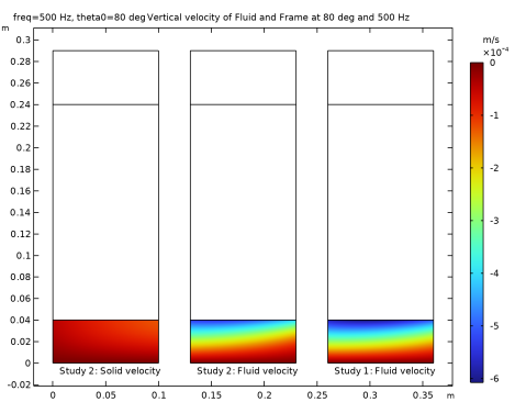
In the Settings window for 2D Plot Group, type Vertical velocity of Fluid and Frame at 80 deg and 500 Hz in the Label text field.
|
|
3
|
Locate the Data section. From the Dataset list, choose Study 2 - Poroelastic Waves/Solution 2 (sol2).
|
|
4
|
|
5
|
|
6
|
|
7
|
|
1
|
|
2
|
|
3
|
|
4
|
|
5
|
|
1
|
|
2
|
|
3
|
|
1
|
|
2
|
|
3
|
|
4
|
|
5
|
|
1
|
In the Model Builder window, right-click Vertical velocity of Fluid and Frame at 80 deg and 500 Hz and choose Annotation.
|
|
2
|
|
3
|
|
4
|
|
5
|
|
6
|
Select the Manual indexing checkbox.
|
|
1
|
|
2
|
|
3
|
|
4
|
|
1
|
|
2
|
|
3
|
|
4
|
|
5
|
|
1
|
In the Model Builder window, right-click Vertical velocity of Fluid and Frame at 80 deg and 500 Hz and choose Duplicate.
|
|
2
|
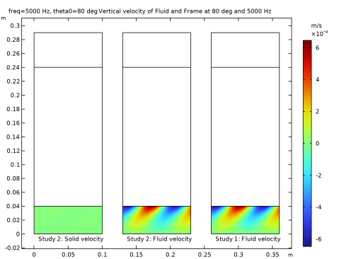
In the Settings window for 2D Plot Group, type Vertical velocity of Fluid and Frame at 80 deg and 5000 Hz in the Label text field.
|
|
3
|
|
1
|
In the Model Builder window, expand the Vertical velocity of Fluid and Frame at 80 deg and 5000 Hz node, then click Surface 3.
|
|
2
|
|
3
|
|
4
|
|
1
|
|
2
|
|
3
|
Locate the Data section. From the Dataset list, choose Study 2 - Poroelastic Waves/Solution 2 (sol2).
|
|
4
|
|
5
|
|
6
|
|
7
|
Locate the Plot Settings section.
|
|
8
|
|
9
|
Select the Two y-axes checkbox.
|
|
10
|
|
1
|
|
2
|
|
3
|
Select the Plot on secondary y-axis checkbox.
|
|
4
|
Locate the y-Axis Data section. In the table, enter the following settings:
|
|
5
|
Select the Unwrap phase checkbox.
|
|
6
|
|
7
|
|
8
|
|
9
|
Click Define custom colors.
|
|
11
|
Click Add to custom colors.
|
|
12
|
|
13
|
|
14
|
|
1
|
|
2
|
|
3
|
|
4
|
|
5
|
|
6
|
Select the Show lines checkbox.
|
|
7
|
|
1
|
|
3
|
|
4
|
|
5
|
|
6
|
Click Define custom colors.
|
|
8
|
Click Add to custom colors.
|
|
9
|
|
10
|
|
1
|
|
2
|
|
3
|
|
4
|
|
5
|
|
6
|
Locate the y-Axis Data section. In the table, enter the following settings:
|
|
7
|
|
8
|
|
9
|
|
1
|
|
2
|
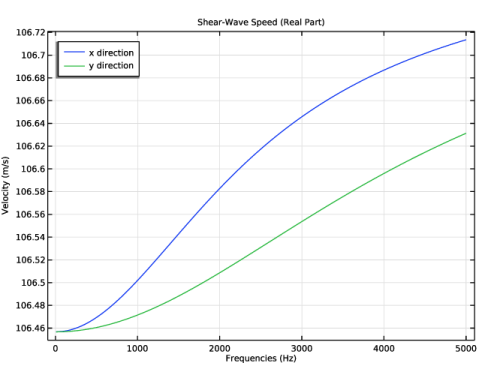
In the Settings window for 1D Plot Group, type Shear-Wave Speed (Real Part) in the Label text field.
|
|
3
|
|
4
|
Locate the Data section. From the Dataset list, choose Study 2 - Poroelastic Waves/Solution 2 (sol2).
|
|
5
|
|
6
|
|
7
|
|
1
|
|
3
|
|
4
|
|
5
|
|
6
|
|
7
|
|
2
|
|
3
|
|
4
|
|
5
|
|
6
|
|
1
|
|
2
|
|
3
|
|
4
|
|
5
|
|
1
|
In the Model Builder window, expand the Shear-Wave Speed (Real Part) 1 node, then click Point Graph 1.
|
|
2
|
|
3
|
|
4
|
Locate the Legends section. In the table, enter the following settings:
|
|
1
|
|
2
|
|
3
|
|
4
|
Locate the Legends section. In the table, enter the following settings:
|
|
1
|
In the Model Builder window, under Results > Shear-Wave Speed (Real Part) 1, Ctrl-click to select Point Graph 1 and Point Graph 2.
|
|
2
|
Right-click and choose Duplicate.
|
|
1
|
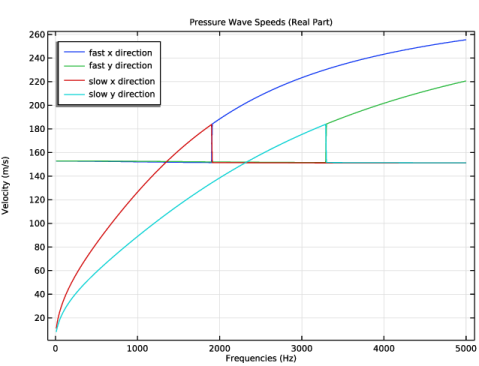
In the Model Builder window, under Results > Pressure Wave Speeds (Real Part), Ctrl-click to select Point Graph 3 and Point Graph 4.
|
|
2
|
|
3
|
|
4
|
Locate the Legends section. In the table, enter the following settings:
|
|
1
|
|
2
|
|
3
|
|
4
|
Locate the Legends section. In the table, enter the following settings:
|
|
5
|