PDF

Active Flame Validation
Introduction
In jet engines and gas turbines, an interaction between the heat release from the flame and the acoustic resonances in the engines can lead to unstable modes that can be damaging to the engine. This occurs because oscillations in the fuel supply results in oscillations in the heat release. The oscillations in the heat release can interfere positively or negatively with the acoustic resonances in the engine such that the oscillations are either dampened or amplified.
To model this effect, it is necessary to have a model of the heat release and how it depends on the acoustic field. This model demonstrates the usage of the domain feature Flame Model in the Pressure Acoustics, Frequency Domain interface with a simple model that can be compared to an analytical solution.
Model Definition
The model consists of a simple 2D geometry, a rectangle with length L, representing a pipe with one closed end and one open end. At the closed end and the two sides, a hard wall boundary condition is used, while at the open end the acoustic pressure is set to zero. In the middle of the rectangle, there is a small domain with an active compact flame. To the left of the flame, the temperature is 300 K and to the right the flame has heated up the air to 1200 K.
The active flame is modeled with the domain feature Flame Model, which adds a heat source in the domain that depends on the acoustic velocity at a reference point. The reference point is set to be on the left boundary of the Flame Model domain. The heat q(x) released by the flame is given by
(1)
where τ(x) is the time-lag, nu(x) is the interaction index, Us is the steady velocity field, and qs is the steady heat release. To ease the analytical modeling of the eigenfrequencies, define the interaction index nu(x) by the parameter n as
(2)
where the specific heat capacity ratio γ and the background pressure p0 are used. Both τ and n are chosen to be independent of the spatial coordinates. The eigenfrequencies can be found analytically as functions of τ and n (see Ref. 1):
(3)
Here, Γ is given as Γ = ρ2c21c1, where the subscript 1 refers to the material parameters to the left of the flame and subscript 2 to those to the right of the flame. The first cosine gives solutions where the active flame does not interfere with the eigenfrequency, while the second parenthesis gives the modes where the active flame impacts the eigenfrequency. The active flame will both shift the resonance frequency either up or down in frequency but it will also dampen or amplify the resonance mode. The damping or amplification is represented by the imaginary part of the eigenfrequency. With the used time convention of exp(iωt) a positive imaginary part represents damping of the mode while a mode with a negative imaginary part is amplified by the active flame. Note the time convention is opposite to the convention used in Ref. 1. A mode that is amplified by the active flame results in an unstable mode. Unstable modes in an engine can be damaging to the engine and they are therefore important to avoid during the design.
Results and Discussion
With an eigenfrequency study step, the first four eigenmodes of the system are found, corresponding to modes with 1/4, 3/4, 5/4, and 7/4 wavelengths in the pipe. The four modes are shown in Figure 1 with the closed end to the left and the open end to the right. Because of the difference in temperature on opposite sides of the active flame, the sound speed and therefore the wavelength is different on each side.
Figure 1: The four lowest eigenmodes of the pipe and active flame.
In Figure 2, the eigenfrequencies are plotted with the real part of the eigenfrequency on the x-axis and the imaginary part on the y-axis. The eigenfrequencies are plotted for both n = 0 (inactive flame) with blue plus signs and n = 5 (active flame) with green plus signs. The theoretical predictions are plotted with circles for both n = 0 and n = 5. It can be seen that all the eigenfrequencies for the inactive flame has zero imaginary part, this is because there is no damping in the system when the flame is inactive. For the second eigenfrequency (at around 700 Hz) the eigenfrequency of the active mode is identical to the eigenfrequency of the passive mode. This mode is not influenced by the active flame and is described by the first cosine in Equation 2.
Figure 2: The real and imaginary part of the eigenfrequencies plotted for the lowest four eigenmodes. The analytical solution plotted with blue circles, the simulations with a passive flame with blue plus signs and the active flame with the green plus signs.
For the first and fourth modes, the imaginary part of the eigenfrequency is positive with the active flame. This means that the modes are dampened by the active flame. This interaction between the acoustic field and the heat released from the flame also reduces the real part of the eigenfrequency. For the third mode, the imaginary part of the eigenfrequency is negative and the mode is amplified by the active flame. The real part of the frequency is shifted upward due to the active flame.
Notes About the COMSOL Implementation
The contribution from the flame model depends nonlinearly on the frequency through the exponential function in Equation 1. Therefore, the model uses the ARPACK nonlinear solver. In the nonlinear solver two settings are changed from the default. The Perform consistency check is turned off, when it is turned an eigenvalue can be returned twice. Secondly, the Eigenvalue scale factor is set to 100 because this is the order of the expected interval between the eigenvalues.
Reference
1. F. Nicoud, L. Benoit, C. Sensiau, and T. Poinsot, “Acoustic modes in combustors with complex impedances and multidimensional active flames,” AIAA J., vol. 45, no. 2,pp. 426–441, 2007.
Application Library path: Acoustics_Module/Tutorials,_Pressure_Acoustics/active_flame_validation
Modeling Instructions
From the File menu, choose New.
New
In the New window, click  Model Wizard.
Model Wizard
1
In the Model Wizard window, click  2D.
2
In the Select Physics tree, select Acoustics > Pressure Acoustics > Pressure Acoustics, Frequency Domain (acpr).
3
Click Add.
4
Click  Study.
5
In the Select Study tree, select General Studies > Eigenfrequency.
6
Global Definitions
Parameters 1
1
In the Model Builder window, under Global Definitions click Parameters 1.
2
In the Settings window for Parameters, locate the Parameters section.
3
Click  Load from File.
4
In the parameter file the analytical eigenfrequencies are calculated. They are calculated iteratively due to the form of the differential equation determining the eigenfrequencies.
Definitions
In the Model Builder window, expand the Component 1 (comp1) > Definitions node.
Geometry 1
Rectangle 1 (r1)
1
In the Model Builder window, expand the Component 1 (comp1) > Geometry 1 node.
2
Right-click Geometry 1 and choose Rectangle.
3
In the Settings window for Rectangle, locate the Size and Shape section.
4
In the Width text field, type L.
5
In the Height text field, type L/10.
6
Click to expand the Layers section. In the table, enter the following settings:
7
Select the Layers to the left checkbox.
8
Clear the Layers on bottom checkbox.
9
Click  Build All Objects.
Add Material
1
In the Materials toolbar, click  Add Material to open the Add Material window.
2
Go to the Add Material window.
3
In the tree, select Built-in > Air.
4
Click the Add to Component button in the window toolbar.
5
In the Materials toolbar, click  Add Material to close the Add Material window.
Definitions
Variables 1
1
In the Model Builder window, under Component 1 (comp1) right-click Definitions and choose Variables.
2
In the Settings window for Variables, locate the Geometric Entity Selection section.
3
From the Geometric entity level list, choose Domain.
4
5
Locate the Variables section. In the table, enter the following settings:
Variables 2
1
In the Model Builder window, right-click Definitions and choose Variables.
2
In the Settings window for Variables, locate the Geometric Entity Selection section.
3
From the Geometric entity level list, choose Domain.
4
5
Locate the Variables section. In the table, enter the following settings:
Pressure Acoustics, Frequency Domain (acpr)
Pressure Acoustics 1
1
In the Model Builder window, under Component 1 (comp1) > Pressure Acoustics, Frequency Domain (acpr) click Pressure Acoustics 1.
2
In the Settings window for Pressure Acoustics, locate the Model Input section.
3
In the T text field, type T_s.
4
In the pA text field, type P_s.
Pressure 1
1
In the Physics toolbar, click  Boundaries and choose Pressure.
2
Flame Model 1
1
In the Physics toolbar, click  Domains and choose Flame Model.
2
3
In the Settings window for Flame Model, locate the Flame Model section.
4
In the nu text field, type n_u.
5
In the τu text field, type tau_u.
6
In the Qs text field, type Q_s.
7
In the Us text field, type u_s.
8
Locate the Acoustic Reference section. From the Acoustic reference list, choose Reference boundary.
9
Locate the Reference Boundary section. Click to select the  Activate Selection toggle button.
10
11
Locate the Acoustic Reference section. Select the Reverse normal direction checkbox.
Mesh 1
1
In the Model Builder window, under Component 1 (comp1) click Mesh 1.
2
In the Settings window for Mesh, locate the Physics-Controlled Mesh section.
3
In the table, clear the Use checkbox for Pressure Acoustics, Frequency Domain (acpr).
4
From the Element size list, choose Extra fine.
5
Click  Build All.
Use the nonlinear eigenvalue solver since the flame model have a nonlinear dependency of the frequency.
Study 1
Step 1: Eigenfrequency
1
In the Model Builder window, under Study 1 click Step 1: Eigenfrequency.
2
In the Settings window for Eigenfrequency, locate the Study Settings section.
3
From the Eigenfrequency solver list, choose ARPACK nonlinear.
4
From the Eigenfrequency search method list, choose Rectangle.
5
In the Approximate number of eigenfrequencies text field, type 5.
6
In the Maximum number of eigenfrequencies text field, type 10.
7
Find the Rectangle search region subsection. In the Smallest real part (Eigenfrequency) text field, type 100.
8
In the Largest real part (Eigenfrequency) text field, type 2000.
9
In the Smallest imaginary part (Eigenfrequency) text field, type -20*n.
10
In the Largest imaginary part (Eigenfrequency) text field, type 20*n.
Set the Eigenvalue scaling factor to 100 as it is the order of the expected difference between the eigenvalues. Perform consistency check is turned off, if it is turned on the solver might return an eigenvalue twice.
11
In the Eigenvalue scaling factor text field, type 100.
12
Clear the Perform consistency check checkbox.
Parametric Sweep
1
In the Study toolbar, click  Parametric Sweep.
Solve for a passive flame (n = 0) and an active flame (n = 5).
2
In the Settings window for Parametric Sweep, locate the Study Settings section.
3
4
5
In the Study toolbar, click  Compute.
Results
Global Evaluation 1
1
In the Model Builder window, expand the Eigenfrequencies (Study 1) node, then click Global Evaluation 1.
2
In the Settings window for Global Evaluation, locate the Expressions section.
3
4
In the Eigenfrequencies (Study 1) toolbar, click  Evaluate.
Numerical and analytical eigenfrequencies
1
In the Results toolbar, click  1D Plot Group.
2
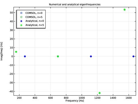
In the Settings window for 1D Plot Group, type Numerical and analytical eigenfrequencies in the Label text field.
3
Click to expand the Title section. From the Title type list, choose Label.
4
Locate the Data section. From the Dataset list, choose Study 1/Parametric Solutions 1 (sol2).
5
From the Parameter selection (n) list, choose First.
6
From the Eigenfrequency selection list, choose First.
7
Locate the Plot Settings section. Select the x-axis label checkbox.
8
Select the y-axis label checkbox.
9
In the x-axis label text field, type Frequency [Hz].
10
In the y-axis label text field, type Imag(freq) [Hz].
11
Locate the Legend section. Select the Show legends checkbox.
12
From the Position list, choose Upper left.
Table Graph 1
1
Right-click Numerical and analytical eigenfrequencies and choose Table Graph.
2
In the Settings window for Table Graph, locate the Data section.
3
From the Source list, choose Evaluation group.
4
From the x-axis data list, choose Eigenfrequency (Hz).
5
From the Plot columns list, choose Manual.
6
In the Columns list box, select Eigenfrequency (Hz).
7
Select the Plot imaginary part checkbox.
8
Locate the Coloring and Style section. Find the Line style subsection. From the Line list, choose None.
9
Find the Line markers subsection. From the Marker list, choose Circle.
10
Click to expand the Legends section. Select the Show legends checkbox.
11
From the Legends list, choose Manual.
12
Filter 1
1
Right-click Table Graph 1 and choose Filter.
2
In the Settings window for Filter, locate the Point Selection section.
3
In the Logical expression for inclusion text field, type col1==0.
Table Graph 2
1
In the Model Builder window, under Results > Numerical and analytical eigenfrequencies right-click Table Graph 1 and choose Duplicate.
2
In the Settings window for Table Graph, locate the Legends section.
3
Filter 1
1
In the Model Builder window, expand the Table Graph 2 node, then click Filter 1.
2
In the Settings window for Filter, locate the Point Selection section.
3
In the Logical expression for inclusion text field, type col1==5.
Numerical and analytical eigenfrequencies
Right-click Results > Numerical and analytical eigenfrequencies > Table Graph 2 > Filter 1 and choose Line Segments.
Line Segments 1
1
In the Settings window for Line Segments, locate the x-Coordinates section.
2
3
Locate the y-Coordinates section. In the table, enter the following settings:
4
Click to expand the Coloring and Style section. Find the Line style subsection. From the Line list, choose None.
5
From the Color list, choose Blue.
6
Find the Line markers subsection. From the Marker list, choose Plus sign.
7
Click to expand the Legends section. Select the Show legends checkbox.
8
From the Legends list, choose Manual.
9
10
In the Numerical and analytical eigenfrequencies toolbar, click  Plot.
Line Segments 2
1
Right-click Results > Numerical and analytical eigenfrequencies > Line Segments 1 and choose Duplicate.
2
In the Settings window for Line Segments, locate the Data section.
3
From the Dataset list, choose Study 1/Parametric Solutions 1 (sol2).
4
From the Parameter selection (n) list, choose Last.
5
From the Eigenfrequency selection list, choose First.
6
Locate the Coloring and Style section. From the Color list, choose Green.
7
Locate the Legends section. In the table, enter the following settings:
8
In the Numerical and analytical eigenfrequencies toolbar, click  Plot.
Rayleigh Criterion
1
In the Results toolbar, click  More Derived Values and choose Average > Surface Average.
2
In the Settings window for Surface Average, locate the Data section.
3
From the Dataset list, choose Study 1/Parametric Solutions 1 (sol2).
4
5
Locate the Expressions section. In the table, enter the following settings:
6
In the Label text field, type Rayleigh Criterion.
7
Click  Evaluate.
Acoustic modes
1
In the Results toolbar, click  2D Plot Group.
2
In the Settings window for 2D Plot Group, click to expand the Title section.
3
From the Title type list, choose Label.
4
Click to expand the Plot Array section. From the Array type list, choose Linear.
5
From the Array axis list, choose y.
6
In the Label text field, type Acoustic modes.
7
Locate the Color Legend section. Clear the Show legends checkbox.
Surface 1
1
Right-click Acoustic modes and choose Surface.
2
In the Settings window for Surface, locate the Data section.
3
From the Dataset list, choose Study 1/Parametric Solutions 1 (sol2).
4
From the Parameter value (n) list, choose 0.
Surface 2
1
Right-click Surface 1 and choose Duplicate.
2
In the Settings window for Surface, locate the Data section.
3
From the Eigenfrequency (Hz) list, choose 694.38.
Surface 3
1
Right-click Surface 2 and choose Duplicate.
2
In the Settings window for Surface, locate the Data section.
3
From the Eigenfrequency (Hz) list, choose 1116.7.
Surface 4
1
Right-click Surface 3 and choose Duplicate.
2
In the Settings window for Surface, locate the Data section.
3
From the Eigenfrequency (Hz) list, choose 1660.8.
4
In the Acoustic modes toolbar, click  Plot.