PDF

Acoustic Streaming in a Microchannel Cross Section
Introduction
Recent advances in the fabrication of microfluidic systems require handling of live cells and other microparticles. One possibility is to use acoustics and exploit the acoustic radiation force to focus particles and/or separate them based on their acoustical properties. When using acoustics in a microchannel, an acoustic streaming flow will be generated and also affect the particles with a viscous drag force; see Ref. 1.
The particle trajectories are determined by the acoustic radiation force and the viscous drag force. The acoustic radiation force is an effect where momentum is transferred from an acoustic field to particles due to nonlinear terms in the governing equations. This results in a net force acting on the particles — the acoustic radiation force.
Due to the nonlinear terms in the Navier–Stokes equations, harmonic perturbation of the flow will lead to a net time-averaged flow called acoustic streaming. Acoustic streaming is a second-order (nonlinear) acoustic effect. The acoustic streaming influences the viscous drag force on the particles. The trajectory of particles in devices are governed by the balance between the viscous drag force (from the streaming flow) and the acoustic radiation force.
There are losses in the acoustic field that produce a heat source. This can be frictional losses in the viscous boundary layers where acoustic energy is transformed into heat, which can result in heating of a microfluidic system.
The model is of a 2D cross section of a microfluidic channel which can, for example, be used for upconcentrating or separating particles in biological fluid samples. This model is based on pressure acoustics and uses effective boundary conditions (the thermoviscous boundary layer impedance or BLI condition) to include the effects of the viscous boundary layers; see Ref. 2.
Model Definition
The model consists of a rectangular fluid domain actuated by vibrating walls; see Figure 1. It is assumed that the surrounding solid is acoustically hard. The model first computes the acoustic field in a Frequency Domain study; then the time-averaged second-order fields, the acoustic streaming flow and acoustic heating in a Stationary study; and lastly the particle trajectories in a Time-dependent study.
The acoustic field is modeled with Pressure Acoustics, Frequency Domain and the Thermoviscous Boundary Layer Impedance is used to account for the damping in the thin viscous boundary layers.
Figure 1: Geometry of the 2D cross section of the microfluidic channel.
The acoustic streaming flow is modeled using the multiphysics couplings Acoustic Streaming Domain Coupling and Acoustic Streaming Boundary Coupling, which from the acoustic field compute and apply the acoustic source terms to the fluid flow interface. The source terms consist of a domain force and a slip velocity on the boundary. The slip velocity includes the contribution from the thin viscous and thermal boundary layers.
The heating from the acoustic field primarily occurs in the viscous boundary layer. The heat generated in the viscous boundary layer is computed analytically (it exists as a predefined variable) and imposed as a boundary layer heat source. To mimic a typical silicon chip with a glass lid, the bottom and the two sides of the rectangle have a constant temperature (due to silicon being a very good heat conductor), while the top is thermally insulating (glass transports heat much less than silicon). Therefore, the temperature will increase at the glass lid, and there will be a temperature gradient across the microfluidic channel.
The particle trajectories are modeled using the Particle Tracing for Fluid Flow interface, which computes the particle trajectories based on the two contributing forces: the acoustic radiation force and the viscous drag force. These two forces depend differently on the size of the particles: for small particles the viscous drag force dominates. whereas the acoustic radiation force dominates for large particles. In most applications, the acoustic radiation force is used to focus particles. This is therefore not possible for particles below a critical particle size, which depends on the material properties of the particle.
Results and Discussion
The system is actuated at the resonance frequency f0 = 1.9652 MHz for the horizontal half-wave resonance. This results in the acoustic field in Figure 2 and an acoustic energy density which is typical for these types of microfluidic devices. The main damping in the system is due to losses in the viscous boundary layers, which therefore determine the Q-factor of the system and the width of the resonance peak. In an actual microfluidic chip there will also be significant damping in the piezoelectric transducer used to actuate the system and in the glue layer. This can widen the resonance peak and lower the resonance frequency.
Figure 2: Acoustic pressure field in the rectangular channel at the horizontal half-wave resonance.
Figure 3: Acoustic streaming flow in the microchannel cross section. The color scale shows amplitude of the fluid flow velocity while the white streaming lines show the direction of the flow field. The streaming consists of the classical four Rayleigh Streaming rolls.
Figure 3 shows the acoustic streaming induced by the acoustic field; the color plot shows the amplitude of the flow field and the white streamlines show the direction of the fluid flow. The streaming flow forms classical Rayleigh streaming rolls, which are typical for boundary-driven streaming. The Rayleigh streaming is induced by the stresses and forces in the viscous boundary layers. In this model, the contributions from the viscous boundary layers are applied as slip velocity and therefore the boundary layers do not have to be numerically resolved.
Figure 4: The temperature field created due to the acoustic heat source in the viscous boundary layers. The white lines represents contour lines of the temperature field.
The heating from the acoustic field induces a temperature gradient across the microchannel. The temperature increase due to the acoustic field is shown in Figure 4. The boundary condition on the acoustic field, Thermoviscous Boundary Layer Impedance, computes the heat generated in the viscous boundary layer in the variable acpr.tvb1.Q_tot. This boundary heat source is used to model the temperature increase in the microfluidic channel. In this example, the acoustic field results in a small temperature increase of the order mK. The temperature increase in an actual microfluidic device will depend on the acoustic field, but also on the thermal properties of the surrounding solid.
Figure 5: The position of particles with radius a = 3 µm at a specific time step. The color of the particles represent the amplitude of their velocity and the lines their trajectory.
The particle trajectory is determined by the acoustic radiation force and the viscous drag force. In Figure 5, the positions of polystyrene particles can be seen at time t = 0.1 s. The color of the particles represents the velocity amplitude and the lines represent the particle trajectory. In Figure 5 the particles have radius a = 3 µm and their trajectories are dominated by the acoustic radiation force focusing the particles in the pressure node. For smaller polystyrene particles with radius a = 0.4 µm, the particle trajectories are shown in Figure 6 at t = 3 s. For the small particles, the viscous drag force dominates; the particles are dragged by the fluid flow, and are not focused in the pressure nodes. The velocities of the small particles are an order of magnitude smaller than those of the large particles.
Figure 6: The position of particles with radius a = 0.4 µm at a time step. The color of the particles represent the amplitude of their velocity and the lines their trajectory.
Notes About the COMSOL Implementation
The implementation is based on pressure acoustics, meaning that the viscous boundary layers are not resolved numerically. Therefore, effective boundary conditions are used to represent the impact of the boundary layers (the Thermoviscous Boundary Layer Impedance condition). This is used for the damping of the acoustic field, slip velocity for the fluid flow, and boundary heat source for the acoustic heating. These are all analytical expressions that are valid when the viscous boundary layer thickness is a lot smaller than the acoustic wavelength and the geometrical length scales; see Ref. 2. Some of the analytical expressions depend on the derivatives at the boundary. Therefore, a thin boundary-layer mesh element is used to improve the accuracy of the normal derivative at the boundary.
References
1. P.B. Muller, R. Barnkob, M.J. Herring Jensen, and H. Bruus, “A numerical study of microparticle acoustophoresis driven by acoustic radiation forces and streaming-induced drag forces,” Lab. Chip., vol. 12, pp. 4617–4627, 2012.
2. J.S. Bach and H. Bruus, “Theory for pressure acoustics with viscous boundary layers and streaming in curved elastic cavities,” J. Acoust. Soc. Am., vol. 144, no. 2, pp. 766–784, 2018.
Application Library path: Acoustics_Module/Nonlinear_Acoustics/acoustic_streaming_microchannel_cross_section
Modeling Instructions
From the File menu, choose New.
New
In the New window, click  Model Wizard.
Model Wizard
1
In the Model Wizard window, click  2D.
2
In the Select Physics tree, select Acoustics > Acoustic Streaming > Acoustic Streaming from Pressure Acoustics.
3
Click Add.
4
In the Select Physics tree, select Heat Transfer > Heat Transfer in Fluids (ht).
5
Click Add.
6
In the Select Physics tree, select Fluid Flow > Particle Tracing > Particle Tracing for Fluid Flow (fpt).
7
Click Add.
8
Click  Study.
9
In the Select Study tree, select Preset Studies for Some Physics Interfaces > Frequency Domain.
10
Global Definitions
Parameters 1
1
In the Model Builder window, under Global Definitions click Parameters 1.
2
In the Settings window for Parameters, locate the Parameters section.
3
Click  Load from File.
4
Browse to the model’s Application Libraries folder and double-click the file acoustic_streaming_microchannel_cross_section_parameters.txt.
Geometry 1
1
In the Model Builder window, under Component 1 (comp1) click Geometry 1.
2
In the Settings window for Geometry, locate the Units section.
3
From the Length unit list, choose mm.
Rectangle 1 (r1)
1
In the Geometry toolbar, click  Rectangle.
2
In the Settings window for Rectangle, locate the Size and Shape section.
3
In the Width text field, type W.
4
In the Height text field, type H.
5
Click  Build All Objects.
Add Material
1
In the Materials toolbar, click  Add Material to open the Add Material window.
2
Go to the Add Material window.
3
In the tree, select Built-in > Water, liquid.
4
Click the Add to Component button in the window toolbar.
5
In the Materials toolbar, click  Add Material to close the Add Material window.
Pressure Acoustics, Frequency Domain (acpr)
Pressure Acoustics 1
1
In the Settings window for Pressure Acoustics, locate the Model Input section.
2
In the T text field, type T0.
Thermoviscous Boundary Layer Impedance 1
1
In the Model Builder window, click Thermoviscous Boundary Layer Impedance 1.
2
In the Settings window for Thermoviscous Boundary Layer Impedance, locate the Fluid Properties section.
3
From the Fluid material list, choose Water, liquid (mat1).
4
Locate the Mechanical Condition section. From the Mechanical condition list, choose Velocity.
5
Specify the v0 vector as
The system is actuated by a boundary velocity in the Thermoviscous Boundary Layer Impedance boundary condition.
Laminar Flow (spf)
1
In the Model Builder window, under Component 1 (comp1) click Laminar Flow (spf).
2
In the Settings window for Laminar Flow, locate the Physical Model section.
3
In the Tref text field, type T0.
To resolve the fluid-flow field on the coarse mesh used for the acoustics, change the discretization.
4
Click to expand the Discretization section. From the Discretization of fluids list, choose P2+P1.
Pressure Point Constraint 1
In the Physics toolbar, click  Points and choose Pressure Point Constraint.
Fluid Properties 1
1
In the Model Builder window, click Fluid Properties 1.
2
In the Settings window for Fluid Properties, locate the Model Input section.
3
From the T list, choose User defined. In the associated text field, type T0.
Pressure Point Constraint 1
1
In the Model Builder window, click Pressure Point Constraint 1.
2
Heat Transfer in Fluids (ht)
In the Model Builder window, under Component 1 (comp1) click Heat Transfer in Fluids (ht).
Temperature 1
1
In the Physics toolbar, click  Boundaries and choose Temperature.
2
3
In the Settings window for Temperature, locate the Temperature section.
4
In the T0 text field, type T0.
Boundary Heat Source 1
1
In the Physics toolbar, click  Boundaries and choose Boundary Heat Source.
2
In the Settings window for Boundary Heat Source, locate the Boundary Heat Source section.
3
From the Qb list, choose Total thermoviscous power dissipation in boundary layers (acpr/tvb1).
4
The boundary heat source acpr.tvb1.Q_tot is the heat source from the acoustically thin boundary layers applied as a boundary heat source.
Particle Tracing for Fluid Flow (fpt)
1
In the Model Builder window, under Component 1 (comp1) click Particle Tracing for Fluid Flow (fpt).
2
In the Settings window for Particle Tracing for Fluid Flow, locate the Particle Release and Propagation section.
3
From the Formulation list, choose Newtonian, ignore inertial terms.
Drag Force 1
1
In the Physics toolbar, click  Domains and choose Drag Force.
2
In the Settings window for Drag Force, locate the Drag Force section.
3
From the u list, choose Lagrangian steady velocity (asdc1).
4
Locate the Model Input section. In the T text field, type T0.
5
Acoustophoretic Radiation Force 1
1
In the Physics toolbar, click  Domains and choose Acoustophoretic Radiation Force.
2
3
In the Settings window for Acoustophoretic Radiation Force, locate the Model Input section.
4
In the T text field, type T0.
5
Locate the Acoustic Fields section. From the p list, choose Acoustic pressure (acpr).
6
From the u list, choose Total acoustic velocity (acpr).
7
Locate the Particle Material Properties section. In the cp,p text field, type cp_p.
8
In the cs,p text field, type cs_p.
Particle Properties 1
1
In the Model Builder window, click Particle Properties 1.
2
In the Settings window for Particle Properties, locate the Particle Properties section.
3
From the ρp list, choose User defined. In the associated text field, type rho_p.
4
In the dp text field, type 2*a.
Release from Grid 1
1
In the Physics toolbar, click  Global and choose Release from Grid.
2
In the Settings window for Release from Grid, locate the Initial Coordinates section.
3
Click  X Range.
4
In the Range dialog, choose Number of values from the Entry method list.
5
In the Start text field, type 10[µm].
6
In the Stop text field, type W-10[µm].
7
In the Number of values text field, type 10.
8
Click Replace.
9
In the Settings window for Release from Grid, locate the Initial Coordinates section.
10
Click  Y Range.
11
In the Range dialog, type 10[µm] in the Start text field.
12
In the Stop text field, type H-10[µm].
13
From the Entry method list, choose Number of values.
14
In the Number of values text field, type 8.
15
Click Replace.
Mesh 1
Free Triangular 1
In the Mesh toolbar, click  Free Triangular.
Boundary Layers 1
1
In the Mesh toolbar, click  Boundary Layers.
2
In the Settings window for Boundary Layers, click to expand the Transition section.
3
Clear the Smooth transition to interior mesh checkbox.
Boundary Layer Properties
1
In the Model Builder window, click Boundary Layer Properties.
2
In the Settings window for Boundary Layer Properties, locate the Boundary Selection section.
3
From the Selection list, choose All boundaries.
4
Locate the Layers section. In the Number of layers text field, type 1.
A single boundary layer ensures accurate normal derivatives on the boundary used for the Acoustic Streaming Boundary Coupling.
5
Click  Build All.
Study 1: Acoustic field
1
In the Model Builder window, click Study 1.
2
In the Settings window for Study, type Study 1: Acoustic field in the Label text field.
3
Locate the Study Settings section. Clear the Generate default plots checkbox.
Step 1: Frequency Domain
1
In the Model Builder window, under Study 1: Acoustic field click Step 1: Frequency Domain.
2
In the Settings window for Frequency Domain, locate the Study Settings section.
3
In the Frequencies text field, type f0.
Add Study
1
In the Home toolbar, click  Add Study to open the Add Study window.
2
Go to the Add Study window.
3
Find the Studies subsection. In the Select Study tree, select Preset Studies for Some Physics Interfaces > Stationary.
4
Click the Add Study button in the window toolbar.
5
In the Select Study tree, select Preset Studies for Some Physics Interfaces > Time Dependent.
6
Click the Add Study button in the window toolbar.
7
In the Home toolbar, click  Add Study to close the Add Study window.
Study 2: Stationary fields
1
In the Settings window for Study, type Study 2: Stationary fields in the Label text field.
2
Locate the Study Settings section. Clear the Generate default plots checkbox.
Step 1: Stationary
1
In the Model Builder window, under Study 2: Stationary fields click Step 1: Stationary.
2
In the Settings window for Stationary, click to expand the Values of Dependent Variables section.
3
Find the Values of variables not solved for subsection. From the Settings list, choose User controlled.
4
From the Method list, choose Solution.
5
From the Study list, choose Study 1: Acoustic field, Frequency Domain.
Study 3: Particle Tracing
1
In the Model Builder window, click Study 3.
2
In the Settings window for Study, type Study 3: Particle Tracing in the Label text field.
Parametric Sweep
1
In the Study toolbar, click  Parametric Sweep.
2
In the Settings window for Parametric Sweep, locate the Study Settings section.
3
4
Step 1: Time Dependent
1
In the Model Builder window, click Step 1: Time Dependent.
2
In the Settings window for Time Dependent, locate the Study Settings section.
3
From the Tolerance list, choose User controlled.
Set the tolerance manually to avoid taking small time steps when the particles are at the pressure node.
4
In the Relative tolerance text field, type 1e-3.
5
In the Output times text field, type range(0,0.02,3).
6
Locate the Physics and Variables Selection section. In the Solve for column of the table, under Component 1 (comp1), clear the checkboxes for Laminar Flow (spf) and Heat Transfer in Fluids (ht).
7
In the Solve for column of the table, under Component 1 (comp1) > Multiphysics, clear the checkboxes for Acoustic Streaming Domain Coupling 1 (asdc1) and Acoustic Streaming Boundary Coupling 1 (asbc1).
8
Click to expand the Values of Dependent Variables section. Find the Values of variables not solved for subsection. From the Settings list, choose User controlled.
9
From the Method list, choose Solution.
10
From the Study list, choose Study 2: Stationary fields, Stationary.
Study 1: Acoustic field
In the Study toolbar, click  Compute.
Study 2: Stationary fields
Click  Compute.
Results
From the Results menu, choose Result Templates.
Result Templates
1
Go to the Result Templates window.
2
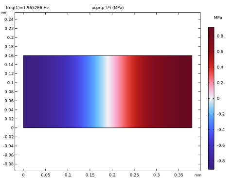
In the tree, select Study 1: Acoustic field/Solution 1 (sol1) > Pressure Acoustics, Frequency Domain > Acoustic Pressure (acpr).
3
Click the Add Result Template button in the window toolbar.
4
From the Results menu, choose Result Templates.
Results
Acoustic Pressure (acpr)
In the Model Builder window, expand the Results node.
Surface 1
1
In the Model Builder window, expand the Acoustic Pressure (acpr) node, then click Surface 1.
2
In the Settings window for Surface, locate the Expression section.
3
In the Expression text field, type acpr.p_t*i.
4
From the Unit list, choose MPa.
5
In the Acoustic Pressure (acpr) toolbar, click  Plot.
Result Templates
1
In the Results toolbar, click  Result Templates to open the Result Templates window.
2
Go to the Result Templates window.
3
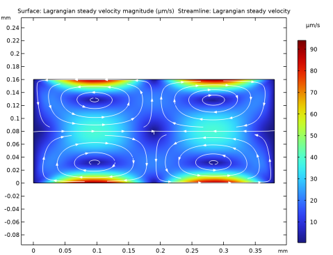
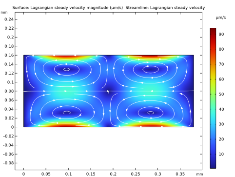
In the tree, select Study 2: Stationary fields/Solution 2 (sol2) > Acoustic Streaming Domain Coupling 1 > Lagrangian Steady Velocity (asdc1).
4
Click the Add Result Template button in the window toolbar.
5
In the Results toolbar, click  Result Templates to close the Result Templates window.
Results
Surface 1
1
In the Model Builder window, expand the Lagrangian Steady Velocity (asdc1) node, then click Surface 1.
2
In the Settings window for Surface, locate the Expression section.
3
From the Unit list, choose µm/s.
4
In the Lagrangian Steady Velocity (asdc1) toolbar, click  Plot.
Result Templates
1
In the Results toolbar, click  Result Templates to open the Result Templates window.
2
Go to the Result Templates window.
3
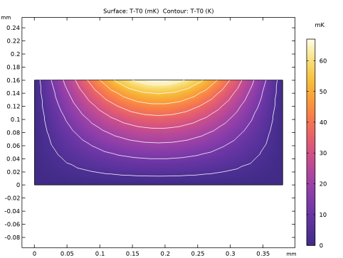
In the tree, select Study 2: Stationary fields/Solution 2 (sol2) > Heat Transfer in Fluids > Temperature (ht).
4
Click the Add Result Template button in the window toolbar.
5
In the Results toolbar, click  Result Templates to close the Result Templates window.
Results
Temperature (ht)
1
In the Settings window for 2D Plot Group, locate the Color Legend section.
2
Select the Show units checkbox.
Surface 1
1
In the Model Builder window, expand the Temperature (ht) node, then click Surface 1.
2
In the Settings window for Surface, locate the Expression section.
3
In the Expression text field, type T-T0.
4
From the Unit list, choose mK.
Contour 1
1
In the Model Builder window, right-click Temperature (ht) and choose Contour.
2
In the Settings window for Contour, locate the Expression section.
3
In the Expression text field, type T-T0.
4
Locate the Levels section. In the Total levels text field, type 8.
5
Locate the Coloring and Style section. From the Coloring list, choose Uniform.
6
From the Color list, choose White.
7
Clear the Color legend checkbox.
8
In the Temperature (ht) toolbar, click  Plot.
Study 3: Particle Tracing
Step 1: Time Dependent
In the Study toolbar, click  Compute.
Results
Particle Trajectories - Large (fpt)
1
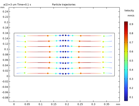
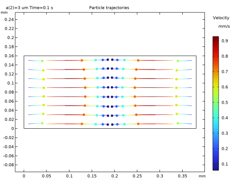
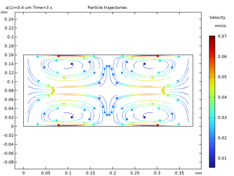
In the Settings window for 2D Plot Group, type Particle Trajectories - Large (fpt) in the Label text field.
2
Locate the Color Legend section. Select the Show units checkbox.
3
Select the Show titles checkbox.
4
Locate the Data section. From the Time (s) list, choose 0.1.
Particle Trajectories 1
1
In the Model Builder window, expand the Particle Trajectories - Large (fpt) node, then click Particle Trajectories 1.
2
In the Settings window for Particle Trajectories, locate the Coloring and Style section.
3
Find the Line style subsection. From the Type list, choose Line.
Color Expression 1
1
In the Model Builder window, expand the Particle Trajectories 1 node, then click Color Expression 1.
2
In the Settings window for Color Expression, locate the Expression section.
3
From the Unit list, choose mm/s.
4
Locate the Coloring and Style section. From the Color table list, choose Rainbow.
5
From the Scale list, choose Linear.
6
In the Color legend title text field, type Velocity.
7
In the Particle Trajectories - Large (fpt) toolbar, click  Plot.
Particle Trajectories - Small (fpt)
1
In the Model Builder window, right-click Particle Trajectories - Large (fpt) and choose Duplicate.
2
In the Settings window for 2D Plot Group, type Particle Trajectories - Small (fpt) in the Label text field.
3
Locate the Data section. From the Parameter value (a (um)) list, choose 0.4.
4
From the Time (s) list, choose 3.
5
In the Particle Trajectories - Small (fpt) toolbar, click  Plot.
Finally, visualize the time-dependent study of the particle trajectories by an animation.
Particle Trajectories
1
In the Results toolbar, click  Animation and choose Player.
2
In the Settings window for Animation, type Particle Trajectories in the Label text field.
3
Locate the Scene section. From the Subject list, choose Particle Trajectories - Large (fpt).
4
Locate the Animation Editing section. From the Parameter value (a (um)) list, choose 3.