|
|
|
|
•
|
A direct solver (PARDISO) is used instead of the default iterative solver. In order to solve a Magnetic Fields problem with a direct solver it is necessary to apply the Gauge Fixing for A-Field feature.
|
|
•
|
The discretization order for the magnetic vector potential A is set to use Linear elements. The discretization order of the Jiles-Atherton auxiliary dependent variables is then automatically set to zero.
|
|
1
|
|
2
|
|
3
|
Click Add.
|
|
4
|
Click
|
|
5
|
In the Select Study tree, select Preset Studies for Selected Physics Interfaces > Coil Geometry Analysis.
|
|
6
|
Click
|
|
1
|
|
2
|
|
11.42 Ω
|
|||
|
1
|
|
2
|
|
1
|
|
2
|
|
3
|
|
4
|
|
1
|
|
2
|
|
3
|
|
4
|
|
5
|
|
6
|
|
1
|
|
2
|
|
3
|
|
4
|
|
5
|
|
6
|
|
7
|
|
1
|
|
2
|
|
3
|
|
4
|
|
5
|
|
6
|
|
7
|
|
1
|
|
2
|
Select the object r1 only.
|
|
3
|
|
4
|
|
5
|
|
1
|
In the Model Builder window, under Component 1 (comp1) > Geometry 1 right-click Work Plane 1 (wp1) and choose Extrude.
|
|
2
|
|
1
|
|
2
|
|
3
|
|
4
|
|
5
|
|
6
|
|
7
|
|
8
|
Click to expand the Layers section. In the table, enter the following settings:
|
|
1
|
|
2
|
|
3
|
|
4
|
|
5
|
|
1
|
|
2
|
Select the object del1 only.
|
|
3
|
|
4
|
|
1
|
|
2
|
|
3
|
|
4
|
|
5
|
|
6
|
|
7
|
|
8
|
|
9
|
|
1
|
|
2
|
|
4
|
|
5
|
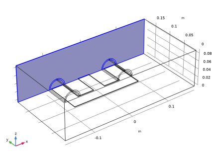
From the Symmetry type for the magnetic flux density list, choose Antisymmetry (all the boundaries at x = 0).
 |
|
1
|
|
3
|
|
4
|
|
1
|
|
2
|
|
3
|
|
4
|
|
5
|
|
6
|
|
7
|
From the list, choose From coil resistance.
|
|
8
|
|
1
|
|
2
|
|
3
|
|
4
|
|
1
|
|
1
|
|
1
|
|
3
|
|
4
|
|
5
|
|
6
|
|
7
|
|
8
|
From the list, choose From coil resistance.
|
|
9
|
|
1
|
|
2
|
|
3
|
|
4
|
|
1
|
|
1
|
|
1
|
|
2
|
|
3
|
|
4
|
|
1
|
In the Model Builder window, under Component 1 (comp1) right-click Materials and choose Blank Material.
|
|
3
|
|
5
|
|
1
|
|
2
|
Go to the Add Material window.
|
|
3
|
|
4
|
Right-click and choose Add to Component 1 (comp1).
|
|
5
|
|
2
|
|
4
|
In the Model Builder window, expand the Jiles–Atherton Hysteretic Material (mat2) node, then click Jiles–Atherton model parameters (ja).
|
|
6
|
Click the Edit button below the table.
|
|
7
|
Choose Diagonal and enter the diagonal elements according to the following table:
|
|
8
|
Click OK.
|
|
1
|
In the Model Builder window, under Component 1 (comp1) > Materials right-click Jiles–Atherton Hysteretic Material (mat2) and choose Rename.
|
|
2
|
In the Rename Material dialog, type Jiles-Atherton Anisotropic Hysteretic Material in the New label text field.
|
|
3
|
Click OK.
|
|
1
|
|
2
|
|
3
|
|
1
|
|
1
|
|
2
|
|
3
|
Click the Custom button.
|
|
4
|
Locate the Element Size Parameters section.
|
|
5
|
|
6
|
|
1
|
|
2
|
|
3
|
|
1
|
|
2
|
|
3
|
|
1
|
|
2
|
|
1
|
|
2
|
|
3
|
|
4
|
|
1
|
|
2
|
|
3
|
In the Model Builder window, expand the Study 1 > Solver Configurations > Solution 1 (sol1) > Dependent Variables 2 node, then click Magnetic Vector Potential (comp1.A).
|
|
4
|
|
5
|
|
6
|
|
1
|
|
1
|
|
2
|
|
3
|
|
5
|
Click
|
|
1
|
In the Model Builder window, under Study 1 > Solver Configurations > Solution 1 (sol1) > Time-Dependent Solver 1 click Fully Coupled 1.
|
|
2
|
|
3
|
|
4
|
In the Model Builder window, under Study 1 > Solver Configurations > Solution 1 (sol1) > Time-Dependent Solver 1 click Direct.
|
|
5
|
|
6
|
|
7
|
|
1
|
|
2
|
|
3
|
|
4
|
Click
|
|
1
|
|
3
|
|
4
|
Select the Lock camera checkbox.
|
|
1
|
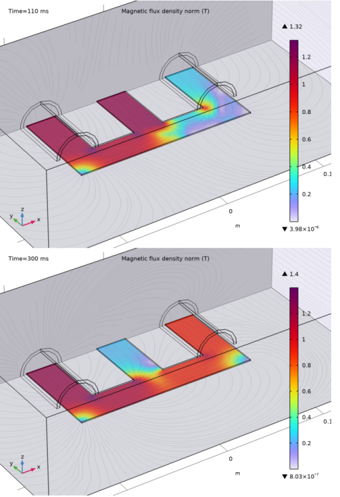
In the Model Builder window, expand the Results > Magnetic Flux Density (mf) node, then click Multislice 1.
|
|
2
|
|
3
|
|
4
|
|
5
|
|
1
|
|
2
|
|
3
|
|
4
|
|
5
|
|
6
|
|
1
|
|
2
|
Click
|
|
3
|
|
4
|
|
5
|
|
1
|
|
2
|
|
3
|
|
4
|
|
5
|
|
1
|
|
2
|
|
3
|
|
1
|
|
3
|
|
4
|
|
1
|
|
2
|
|
3
|
|
1
|
|
2
|
|
3
|
|
4
|
|
5
|
|
6
|
|
1
|
|
2
|
|
3
|
|
4
|
|
5
|
|
6
|
|
1
|
|
2
|
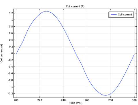
In the Settings window for Global, click Replace Expression in the upper-right corner of the y-Axis Data section. From the menu, choose Component 1 (comp1) > Magnetic Fields > Coil parameters > mf.ICoil_1 - Coil current - A.
|
|
1
|
|
2
|
|
3
|
|
4
|
Click
|
|
5
|
|
6
|
|
7
|
|
8
|
Click Replace.
|
|
9
|
|
10
|
|
1
|
|
2
|
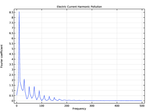
In the Settings window for 1D Plot Group, type Electric Current Harmonic Pollution in the Label text field.
|
|
3
|
|
4
|
|
1
|
|
2
|
|
3
|
|
4
|
|
5
|
|
1
|
|
2
|
|
3
|
|
4
|
|
5
|
|
6
|
Click
|
|
7
|
|
8
|
|
9
|
|
10
|
Click Replace.
|
|
1
|
|
2
|
|
4
|
|
5
|
|
6
|
|
1
|
|
2
|
|
1
|
|
2
|
|
3
|
|
4
|
|
1
|
|
2
|
|
3
|
|
4
|
|
5
|
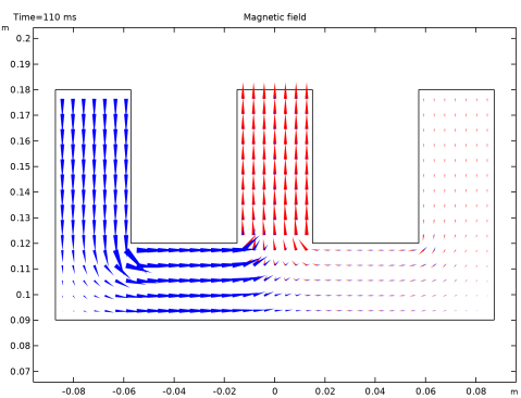
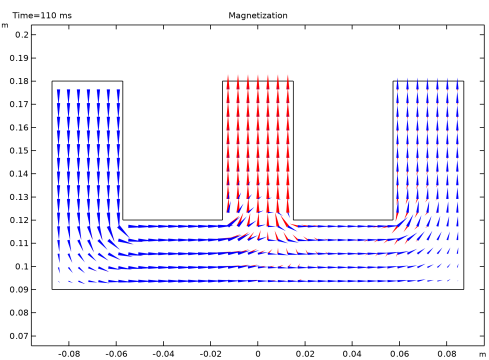
Locate the Arrow Positioning section. Find the x grid points subsection. In the Points text field, type 41.
|
|
6
|
|
1
|
|
2
|
|
3
|
|
4
|
|
5
|
|
6
|
|
1
|
|
2
|
|
3
|
|
4
|
|
1
|
|
2
|
|
1
|
|
2
|
|
3
|
|
4
|
Click OK.
|
|
1
|
|
2
|
|
3
|
|
4
|
|
5
|
|
1
|
|
2
|
|
3
|
|
4
|
|
5
|
|
6
|
|
1
|
|
2
|
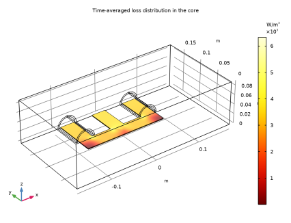
In the Settings window for 3D Plot Group, type Averaged Losses over the Last Period in the Label text field.
|
|
1
|
|
2
|
|
3
|
|
4
|
|
1
|
|
2
|
|
3
|
|
4
|
|
5
|
|
6
|
|
1
|
In the Model Builder window, under Results > Averaged Losses over the Last Period > Volume 1 click Selection 1.
|
|
2
|
|
3
|
Click to select the
|
|
4
|
|
6
|
Click
|
|
8
|
|
1
|
|
2
|
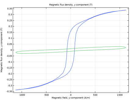
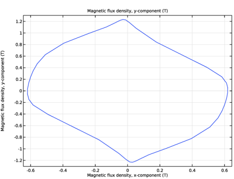
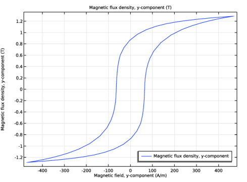
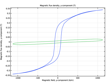
In the Settings window for 1D Plot Group, type Two Different Hysteresis Loops for Two Different Locations in the Label text field.
|
|
3
|
|
4
|
|
1
|
|
2
|
|
3
|
|
4
|
|
5
|
Click to select the
|
|
7
|
|
8
|
|
9
|
|
10
|
|
11
|
Click to expand the Legends section. In the Two Different Hysteresis Loops for Two Different Locations toolbar, click
 |
|
1
|
|
2
|
|
3
|
|
4
|
|
5
|
|
6
|
Locate the Expressions section. In the table, enter the following settings:
|
|
7
|