PDF

Tubular Permanent Magnet Generator
Introduction
This tutorial demonstrates how to model a tubular permanent magnet generator in a 2D axisymmetric system. This is accomplished by coupling the Magnetic Fields interface with a Moving Mesh. Note: for rotational electrical machines, the Rotating Machinery, Magnetic interface is the recommended method. As the tubular generator is a type of linear motor, this can be modeled using a 2D axisymmetric geometry and applying periodic conditions on the appropriate boundaries.
This tubular generator model considers an array of magnetics moving with a constant velocity through a tube of open circuit-connected three phase coils in the stator. The model results show the magnetic fields in the system with the key result being the calculated induced voltages from the generator. This can be the basis for then applying a proper current.
Model Definition
The geometry consists of two parts, the stationary stator and the moving slider. The stator consists of three coils running three different phases. The slider contains an array of cylindrical magnets with alternating polarities separated by nonlinear magnetic material, see Figure 1. The slider is modeled using a Moving Mesh and is connected to the stator using a Periodic Magnetic Continuity boundary pair.
As the tubular generator consists of a periodic array of magnets and coils, symmetry can be utilized to reduce computational cost. Here, only one unit cell of the structure is modeled and a periodic condition is applied to the top and bottom boundaries of the geometry to represent the rest of the array. This is done by applying continuous Periodic Conditions to the edges of the slider and stator.
The study step of this model is divided into two parts. An initial stationary study to get the initial condition followed by a time dependent study to analyze the induced voltages as the slider moves through the stator.
Figure 1: Left: 3D view of the tubular generator showing the magnetic flux density in the nonlinear magnetic material. Right: 2D cross-sectional axisymmetric view of the tubular generator. This shows the arrangements of the coils, the permanent magnets, and the nonlinear magnetic material. The left “Slider” section of the geometry is mapped using a moving mesh while the right “Stator” section uses a fixed mesh. These two meshes communicate through the applied periodic magnetic continuity boundary pair. The red periodic boundaries apply a repeating functionality allowing for the representation of a larger geometry.
Results and Discussion
This model produces results in both 2D cross-sectional and revolved views. Figure 2 shows the cross-sectional magnetic flux in the generator where the field lines show the continuity across the periodic conditions. In Figure 3, the geometry is partially revolved to show the 3D nature of the tubular generator with a section left out to show the internal magnetic vector potential in the nonlinear iron. Finally, Figure 4 shows the voltage induced by the generator in each of the three coil phases.
Several of the key variables for the performance of the motor are set in the Parameters sections of the model. This allows for convenient changing of variables such as the slider speed and the number of turns in the coils to experiment with and produce different voltage curves from the generator.
Figure 2: Cross-sectional view of the magnetic flux in the tubular generator. Three of the modeled unit cells are stacked together to illustrate the periodic nature of the system.
Figure 3: Revolved representation of the 2D simulation showing the magnetic vector potential in the nonlinear magnetic material in both the slider and the stator. This plot shows three stacked copies of the modeled geometry to represent a larger section of the linear generator. This illustrates how the periodic conditions knit the vector potentials together at the boundaries of the geometry.
Figure 4: Open circuit voltages produced in each of the three phases of coils.
Application Library path: ACDC_Module/Devices,_Motors_and_Generators/tubular_permanent_magnet_generator
Modeling Instructions
From the File menu, choose New.
New
In the New window, click  Model Wizard.
Model Wizard
1
In the Model Wizard window, click  2D Axisymmetric.
2
In the Select Physics tree, select AC/DC > Electromagnetic Fields > Magnetic Fields (mf).
3
Click Add.
4
In the Select Physics tree, select Mathematics > Deformed Mesh > Moving Mesh > Prescribed Deformation.
5
Click Add.
6
Click  Study.
7
In the Select Study tree, select General Studies > Stationary.
8
Global Definitions
Parameters 1
1
In the Model Builder window, under Global Definitions click Parameters 1.
2
In the Settings window for Parameters, locate the Parameters section.
3
Click the Load button. From the menu, choose Load from File.
4
Geometry 1
1
In the Model Builder window, under Component 1 (comp1) click Geometry 1.
2
In the Settings window for Geometry, locate the Units section.
3
From the Length unit list, choose mm.
4
Locate the Advanced section. From the Default repair tolerance list, choose Relative.
Rectangle 1 (r1)
1
In the Geometry toolbar, click  Rectangle.
2
In the Settings window for Rectangle, locate the Size and Shape section.
3
In the Width text field, type M_w.
4
In the Height text field, type P_P.
5
Locate the Position section. In the r text field, type S_r.
6
Click to expand the Layers section. In the table, enter the following settings:
7
Select the Layers on top checkbox.
Rectangle 2 (r2)
1
In the Geometry toolbar, click  Rectangle.
2
In the Settings window for Rectangle, locate the Size and Shape section.
3
In the Width text field, type Sl_tw.
4
In the Height text field, type Sl_h.
5
Locate the Position section. In the r text field, type S_r+M_w.
6
In the z text field, type Mg_h/2-(Sl_h-Sl_ch)/2.
Move 1 (mov1)
1
In the Geometry toolbar, click  Transforms and choose Move.
2
3
In the Settings window for Move, locate the Input section.
4
Select the Keep input objects checkbox.
5
Locate the Displacement section. In the z text field, type Mg_h+Sl_ch.
Rectangle 3 (r3)
1
In the Geometry toolbar, click  Rectangle.
2
In the Settings window for Rectangle, locate the Size and Shape section.
3
In the Width text field, type M_w.
4
In the Height text field, type P_P.
5
Locate the Position section. In the r text field, type S_r+M_w+Sl_tw+A_g+St_w.
6
Locate the Layers section. In the table, enter the following settings:
7
Select the Layers on top checkbox.
Rectangle 4 (r4)
1
In the Geometry toolbar, click  Rectangle.
2
In the Settings window for Rectangle, locate the Size and Shape section.
3
In the Width text field, type St_w.
4
In the Height text field, type St_h*1.5.
5
Locate the Position section. In the r text field, type S_r+M_w+Sl_tw+A_g.
6
In the z text field, type St_h+C_h-St_h*1.5/2.
Move 2 (mov2)
1
In the Geometry toolbar, click  Transforms and choose Move.
2
3
In the Settings window for Move, locate the Input section.
4
Select the Keep input objects checkbox.
5
Locate the Displacement section. In the z text field, type C_h+St_h.
Rectangle 5 (r5)
1
In the Geometry toolbar, click  Rectangle.
2
In the Settings window for Rectangle, locate the Size and Shape section.
3
In the Width text field, type St_w.
4
In the Height text field, type St_h*1.5/2.
5
Locate the Position section. In the r text field, type S_r+M_w+Sl_tw+A_g.
Rectangle 6 (r6)
1
In the Geometry toolbar, click  Rectangle.
2
In the Settings window for Rectangle, locate the Size and Shape section.
3
In the Width text field, type St_w.
4
In the Height text field, type St_h*1.5/2.
5
Locate the Position section. In the r text field, type S_r+M_w+Sl_tw+A_g.
6
In the z text field, type P_P-1.5*St_h/2.
Fillet 1 (fil1)
1
In the Geometry toolbar, click  Fillet.
2
On the object mov2, select Points 1 and 4 only.
3
On the object r4, select Points 1 and 4 only.
4
On the object r5, select Point 4 only.
5
On the object r6, select Point 1 only.
6
In the Settings window for Fillet, locate the Radius section.
7
In the Radius text field, type A_g.
Rectangle 7 (r7)
1
In the Geometry toolbar, click  Rectangle.
2
In the Settings window for Rectangle, locate the Size and Shape section.
3
In the Width text field, type S_r+M_w+Sl_tw+A_g/2.
4
In the Height text field, type P_P.
Rectangle 8 (r8)
1
In the Geometry toolbar, click  Rectangle.
2
In the Settings window for Rectangle, locate the Size and Shape section.
3
In the Width text field, type 50.
4
In the Height text field, type P_P.
5
Locate the Position section. In the r text field, type S_r+M_w+Sl_tw+A_g/2.
6
Locate the Layers section. In the table, enter the following settings:
7
Clear the Layers on bottom checkbox.
8
Select the Layers to the left checkbox.
Moving Part
1
In the Geometry toolbar, click  Booleans and Partitions and choose Union.
2
In the Settings window for Union, type Moving Part in the Label text field.
3
Select the objects mov1, r1, r2, and r7 only.
4
Locate the Selections of Resulting Entities section. Select the Resulting objects selection checkbox.
Statoric Part
1
In the Geometry toolbar, click  Booleans and Partitions and choose Union.
2
In the Settings window for Union, type Statoric Part in the Label text field.
3
Select the objects fil1(1), fil1(2), fil1(3), fil1(4), r3, and r8 only.
4
Locate the Selections of Resulting Entities section. Select the Resulting objects selection checkbox.
Magnets
1
In the Geometry toolbar, click  Selections and choose Explicit Selection.
2
In the Settings window for Explicit Selection, type Magnets in the Label text field.
3
On the object uni1, select Domains 2, 4, and 6 only.
Laminated Core
1
In the Geometry toolbar, click  Selections and choose Explicit Selection.
2
In the Settings window for Explicit Selection, type Laminated Core in the Label text field.
3
On the object uni1, select Domains 3, 5, 8, and 9 only.
4
On the object uni2, select Domains 2–6, 8, 10, 12, and 13 only.
Coils
1
In the Geometry toolbar, click  Selections and choose Explicit Selection.
2
In the Settings window for Explicit Selection, type Coils in the Label text field.
3
On the object uni2, select Domains 7, 9, and 11 only.
Form Union (fin)
1
In the Model Builder window, under Component 1 (comp1) > Geometry 1 click Form Union (fin).
2
In the Settings window for Form Union/Assembly, locate the Form Union/Assembly section.
3
From the Action list, choose Form an assembly.
4
From the Repair tolerance list, choose Relative.
5
Click the  Zoom Extents button in the Graphics toolbar.
6
In the Geometry toolbar, click  Build All.
The geometry should look like the figure above.
Add Material
1
In the Materials toolbar, click  Add Material to open the Add Material window.
2
Go to the Add Material window.
3
In the tree, select AC/DC > Soft Iron (Without Losses).
4
Click the Add to Component button in the window toolbar.
Materials
Soft Iron (Without Losses) (mat1)
1
In the Settings window for Material, locate the Geometric Entity Selection section.
2
From the Selection list, choose Laminated Core.
Add Material
1
Go to the Add Material window.
2
In the tree, select AC/DC > Hard Magnetic Materials > Sintered NdFeB Grades (Chinese Standard) > N50 (Sintered NdFeB).
3
Click the Add to Component button in the window toolbar.
Materials
N50 (Sintered NdFeB) (mat2)
1
In the Settings window for Material, locate the Geometric Entity Selection section.
2
From the Selection list, choose Magnets.
Add Material
1
Go to the Add Material window.
2
In the tree, select AC/DC > Copper.
3
Click the Add to Component button in the window toolbar.
4
In the Materials toolbar, click  Add Material to close the Add Material window.
Materials
Copper (mat3)
1
In the Settings window for Material, locate the Geometric Entity Selection section.
2
From the Selection list, choose Coils.
Moving Mesh
Prescribed Deformation 1
The Moving Mesh models the linear motion of the slider.
1
In the Model Builder window, under Component 1 (comp1) > Moving Mesh click Prescribed Deformation 1.
2
In the Settings window for Prescribed Deformation, locate the Geometric Entity Selection section.
3
From the Selection list, choose Moving Part.
4
Locate the Prescribed Deformation section. Specify the dx vector as
Magnetic Fields (mf)
Free Space 1
1
In the Model Builder window, under Component 1 (comp1) > Magnetic Fields (mf) click Free Space 1.
2
In the Settings window for Free Space, locate the Stabilization section.
3
From the σstab list, choose Automatic.
Domain Coil 1
1
In the Physics toolbar, click  Domains and choose Domain Coil.
2
3
In the Settings window for Domain Coil, locate the Coil section.
4
From the Conductor model list, choose Homogenized multiturn.
5
In the Icoil text field, type 0[A].
6
Locate the Homogenized Conductor section. In the N text field, type Nturns.
7
From the Coil wire cross-section area list, choose Filling factor.
8
In the f text field, type 0.8.
Domain Coil 3
Right-click Domain Coil 1 and choose Split by Connectivity.
Magnet 1
1
In the Physics toolbar, click  Domains and choose Magnet.
2
3
In the Settings window for Magnet, locate the Constitutive Relation Jc-E section.
4
From the Constrain for induced currents list, choose No induced currents constrain.
North 1
1
In the Model Builder window, click North 1.
2
South 1
1
In the Model Builder window, click South 1.
2
Laminated Core
1
In the Physics toolbar, click  Domains and choose Ampère’s Law in Solids.
2
In the Settings window for Ampère’s Law in Solids, type Laminated Core in the Label text field.
3
Locate the Domain Selection section. From the Selection list, choose Laminated Core.
4
Locate the Constitutive Relation B-H section. From the Magnetization model list, choose B-H curve.
Periodic Condition 1
1
In the Physics toolbar, click  Boundaries and choose Periodic Condition.
2
Periodic Condition 2
1
In the Physics toolbar, click  Boundaries and choose Periodic Condition.
2
Periodic Magnetic Continuity 1
1
In the Physics toolbar, click  Pairs and choose Periodic Magnetic Continuity.
2
In the Settings window for Periodic Magnetic Continuity, locate the Pair Selection section.
3
4
In the Add dialog, select Identity Boundary Pair 1 (ap1) in the Pairs list.
5
Mesh 1
1
In the Model Builder window, under Component 1 (comp1) right-click Mesh 1 and choose Build All.
2
Click the  Zoom Extents button in the Graphics toolbar.
The mesh should look like the figure above.
Study 1
Step 2: Time Dependent
1
In the Study toolbar, click  Time Dependent.
2
In the Settings window for Time Dependent, locate the Study Settings section.
3
In the Output times text field, type range(0,0.02,1.5)*P_P/speed.
Solution 1 (sol1)
1
In the Study toolbar, click  Show Default Solver.
2
In the Model Builder window, expand the Solution 1 (sol1) node.
3
In the Model Builder window, expand the Study 1 > Solver Configurations > Solution 1 (sol1) > Time-Dependent Solver 1 node, then click Fully Coupled 1.
4
In the Settings window for Fully Coupled, click to expand the Method and Termination section.
5
From the Jacobian update list, choose On every iteration.
6
In the Study toolbar, click  Compute.
Results
Revolution 2D 1
In the Model Builder window, expand the Results > Datasets node, then click Revolution 2D 1.
Selection
1
In the Results toolbar, click  Attributes and choose Selection.
2
In the Settings window for Selection, locate the Geometric Entity Selection section.
3
From the Geometric entity level list, choose Domain.
4
Click  Paste Selection.
5
In the Paste Selection dialog, type 3, 5, 8, 9, 11-15, 17, 19, 21, 22 in the Selection text field.
6
Revolution 2D 2
1
In the Results toolbar, click  More Datasets and choose Revolution 2D.
2
In the Settings window for Revolution 2D, click to expand the Revolution Layers section.
3
In the Start angle text field, type -90.
4
In the Revolution angle text field, type 225.
Selection
1
In the Results toolbar, click  Attributes and choose Selection.
2
In the Settings window for Selection, locate the Geometric Entity Selection section.
3
From the Geometric entity level list, choose Domain.
4
From the Selection list, choose Magnets.
Revolution 2D 3
1
In the Results toolbar, click  More Datasets and choose Revolution 2D.
2
In the Settings window for Revolution 2D, locate the Revolution Layers section.
3
In the Start angle text field, type -90.
4
In the Revolution angle text field, type 225.
Selection
1
In the Results toolbar, click  Attributes and choose Selection.
2
In the Settings window for Selection, locate the Geometric Entity Selection section.
3
From the Geometric entity level list, choose Domain.
4
From the Selection list, choose Coils.
Magnetic Flux Density (mf)
1
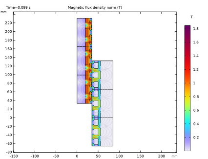
In the Model Builder window, expand the Results > Magnetic Flux Density (mf) node, then click Magnetic Flux Density (mf).
2
In the Settings window for 2D Plot Group, locate the Color Legend section.
3
Clear the Show maximum and minimum values checkbox.
4
Select the Show units checkbox.
Contour 1
1
In the Model Builder window, click Contour 1.
2
In the Settings window for Contour, locate the Expression section.
3
In the Expression text field, type r*mf.Aphi.
Color Expression 1
1
Right-click Contour 1 and choose Color Expression.
2
In the Settings window for Color Expression, locate the Coloring and Style section.
3
Clear the Color legend checkbox.
Surface 2
1
In the Model Builder window, under Results > Magnetic Flux Density (mf) right-click Surface 1 and choose Duplicate.
2
In the Settings window for Surface, click to expand the Title section.
3
From the Title type list, choose None.
4
Locate the Coloring and Style section. Clear the Color legend checkbox.
Transformation 1
1
Right-click Surface 2 and choose Transformation.
2
In the Settings window for Transformation, locate the Transformation section.
3
In the z text field, type P_P.
Surface 3
In the Model Builder window, under Results > Magnetic Flux Density (mf) right-click Surface 2 and choose Duplicate.
Transformation 1
1
In the Model Builder window, expand the Surface 3 node, then click Transformation 1.
2
In the Settings window for Transformation, locate the Transformation section.
3
In the z text field, type -P_P.
Streamline 2
In the Model Builder window, under Results > Magnetic Flux Density (mf) right-click Streamline 1 and choose Duplicate.
Transformation 1
1
In the Model Builder window, expand the Streamline 2 node.
2
Right-click Streamline 2 and choose Transformation.
3
In the Settings window for Transformation, locate the Transformation section.
4
In the z text field, type P_P.
Streamline 3
In the Model Builder window, under Results > Magnetic Flux Density (mf) right-click Streamline 2 and choose Duplicate.
Transformation 1
1
In the Model Builder window, expand the Streamline 3 node, then click Transformation 1.
2
In the Settings window for Transformation, locate the Transformation section.
3
In the z text field, type -P_P.
Contour 2
In the Model Builder window, under Results > Magnetic Flux Density (mf) right-click Contour 1 and choose Duplicate.
Transformation 1
1
In the Model Builder window, expand the Contour 2 node.
2
Right-click Contour 2 and choose Transformation.
3
In the Settings window for Transformation, locate the Transformation section.
4
In the z text field, type P_P.
Contour 3
In the Model Builder window, under Results > Magnetic Flux Density (mf) right-click Contour 2 and choose Duplicate.
Transformation 1
1
In the Model Builder window, expand the Contour 3 node, then click Transformation 1.
2
In the Settings window for Transformation, locate the Transformation section.
3
In the z text field, type -P_P.
4
In the Magnetic Flux Density (mf) toolbar, click  Plot.
5
Click the  Zoom Extents button in the Graphics toolbar.
Magnetic Flux Density Norm, Revolved Geometry (mf)
1
In the Model Builder window, under Results click Magnetic Flux Density, Revolved Geometry (mf).
2
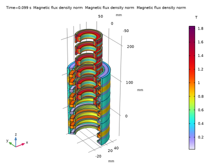
In the Settings window for 3D Plot Group, type Magnetic Flux Density Norm, Revolved Geometry (mf) in the Label text field.
3
Locate the Data section. From the Time (s) list, choose Interpolation.
4
Click to expand the Title section. From the Title type list, choose Custom.
5
Find the Type and data subsection. Clear the Type checkbox.
6
Clear the Unit checkbox.
7
Locate the Color Legend section. Clear the Show maximum and minimum values checkbox.
8
Select the Show units checkbox.
Contour 1
1
In the Model Builder window, expand the Magnetic Flux Density Norm, Revolved Geometry (mf) node, then click Contour 1.
2
In the Settings window for Contour, locate the Expression section.
3
In the Expression text field, type mf.normB.
Filter 1
1
In the Model Builder window, expand the Contour 1 node.
2
Right-click Filter 1 and choose Disable.
Volume 2
1
In the Model Builder window, under Results > Magnetic Flux Density Norm, Revolved Geometry (mf) right-click Volume 1 and choose Duplicate.
2
In the Settings window for Volume, locate the Coloring and Style section.
3
Clear the Color legend checkbox.
Transformation 1
1
Right-click Volume 2 and choose Transformation.
2
In the Settings window for Transformation, locate the Transformation section.
3
In the z text field, type P_P.
Volume 3
In the Model Builder window, under Results > Magnetic Flux Density Norm, Revolved Geometry (mf) right-click Volume 2 and choose Duplicate.
Transformation 1
1
In the Model Builder window, expand the Volume 3 node, then click Transformation 1.
2
In the Settings window for Transformation, locate the Transformation section.
3
In the z text field, type -P_P.
Contour 2
In the Model Builder window, under Results > Magnetic Flux Density Norm, Revolved Geometry (mf) right-click Contour 1 and choose Duplicate.
Transformation 1
1
In the Model Builder window, right-click Contour 2 and choose Transformation.
2
In the Settings window for Transformation, locate the Transformation section.
3
In the z text field, type P_P.
Contour 3
In the Model Builder window, under Results > Magnetic Flux Density Norm, Revolved Geometry (mf) right-click Contour 2 and choose Duplicate.
Transformation 1
1
In the Model Builder window, expand the Contour 3 node, then click Transformation 1.
2
In the Settings window for Transformation, locate the Transformation section.
3
In the z text field, type -P_P.
4
In the Magnetic Flux Density Norm, Revolved Geometry (mf) toolbar, click  Plot.
5
Click the  Zoom Extents button in the Graphics toolbar.
Magnetic Vector Potential
1
In the Results toolbar, click  3D Plot Group.
2
In the Settings window for 3D Plot Group, type Magnetic Vector Potential in the Label text field.
3
Locate the Title section. From the Title type list, choose Label.
Magnetic vector potential
1
Right-click Magnetic Vector Potential and choose Surface.
2
In the Settings window for Surface, type Magnetic vector potential in the Label text field.
3
Locate the Expression section. In the Expression text field, type mf.Aphi.
4
Locate the Coloring and Style section. From the Color table type list, choose Discrete.
5
In the Number of bands text field, type 21.
6
Click the  Zoom Extents button in the Graphics toolbar.
Magnetic vector potential Translated Up
1
Right-click Magnetic vector potential and choose Duplicate.
2
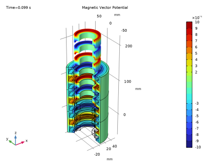
In the Settings window for Surface, type Magnetic vector potential Translated Up in the Label text field.
3
Locate the Coloring and Style section. Clear the Color legend checkbox.
Transformation 1
1
Right-click Magnetic vector potential Translated Up and choose Transformation.
2
In the Settings window for Transformation, locate the Transformation section.
3
In the z text field, type P_P.
Magnetic vector potential Translated Down
1
In the Model Builder window, right-click Magnetic vector potential Translated Up and choose Duplicate.
2
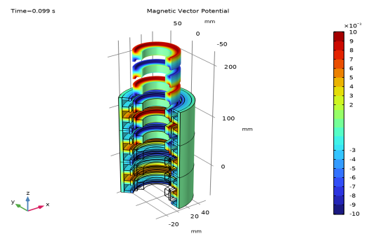
In the Settings window for Surface, type Magnetic vector potential Translated Down in the Label text field.
Transformation 1
1
In the Model Builder window, expand the Magnetic vector potential Translated Down node, then click Transformation 1.
2
In the Settings window for Transformation, locate the Transformation section.
3
In the z text field, type -P_P.
4
Click the  Zoom Extents button in the Graphics toolbar.
5
In the Magnetic Vector Potential toolbar, click  Plot.
Phase Voltages
1
In the Results toolbar, click  1D Plot Group.
2
In the Settings window for 1D Plot Group, type Phase Voltages in the Label text field.
Phase Voltages
1
Right-click Phase Voltages and choose Global.
2
In the Settings window for Global, type Phase Voltages in the Label text field.
3
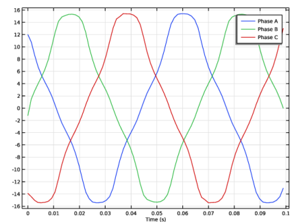
Locate the y-Axis Data section. In the table, enter the following settings:
4
In the Phase Voltages toolbar, click  Plot.