|
|
|
|
1
|
|
2
|
|
3
|
Click Add.
|
|
4
|
Click
|
|
5
|
|
6
|
Click
|
|
1
|
|
2
|
|
1
|
|
2
|
|
3
|
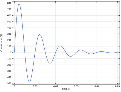
Locate the Definition section. In the Expression text field, type sin(2*pi*fc*t)*exp(-t/period)*1000.
|
|
4
|
|
5
|
|
6
|
Click
|
|
1
|
|
2
|
|
3
|
|
4
|
|
5
|
|
6
|
Locate the Selections of Resulting Entities section. Select the Resulting objects selection checkbox.
|
|
1
|
|
2
|
|
3
|
|
4
|
|
5
|
|
6
|
Locate the Selections of Resulting Entities section. Select the Resulting objects selection checkbox.
|
|
1
|
|
2
|
|
3
|
|
4
|
|
5
|
|
6
|
|
7
|
Locate the Selections of Resulting Entities section. Select the Resulting objects selection checkbox.
|
|
1
|
|
2
|
|
3
|
|
4
|
|
5
|
|
6
|
|
7
|
Locate the Selections of Resulting Entities section. Select the Resulting objects selection checkbox.
|
|
1
|
|
2
|
|
3
|
|
4
|
|
5
|
Locate the Selections of Resulting Entities section. Select the Resulting objects selection checkbox.
|
|
1
|
|
2
|
|
1
|
|
2
|
|
1
|
|
2
|
|
3
|
Click to expand the Discretization section.
|
|
1
|
|
3
|
In the Settings window for Transition Boundary Condition, locate the Transition Boundary Condition section.
|
|
4
|
From the εrb list, choose User defined. From the μrb list, choose User defined. In the associated text field, type mur.
|
|
5
|
|
6
|
|
1
|
|
3
|
In the Settings window for Line Current (Out-of-Plane), locate the Line Current (Out-of-Plane) section.
|
|
4
|
|
1
|
|
3
|
|
1
|
In the Model Builder window, right-click TBC in the Frequency Domain (comp1) and choose Paste Magnetic Fields.
|
|
2
|
|
3
|
|
1
|
In the Model Builder window, expand the TBC in the Frequency Domain (comp1) > Thick Layer (mf2) node, then click Transition Boundary Condition 1.
|
|
2
|
In the Settings window for Transition Boundary Condition, locate the Transition Boundary Condition section.
|
|
3
|
|
4
|
|
5
|
|
6
|
Click Approximation in the upper-right corner of the Time Domain and Eigenfrequency section. From the menu, choose Compute Approximation.
|
|
1
|
In the Model Builder window, right-click TBC in the Frequency Domain (comp1) and choose Paste Magnetic Fields.
|
|
2
|
|
3
|
|
1
|
In the Model Builder window, expand the TBC in the Frequency Domain (comp1) > Very Thin Layer (mf3) node, then click Transition Boundary Condition 1.
|
|
2
|
In the Settings window for Transition Boundary Condition, locate the Transition Boundary Condition section.
|
|
3
|
|
1
|
|
2
|
|
3
|
|
4
|
|
1
|
|
2
|
|
3
|
|
4
|
|
5
|
|
1
|
|
2
|
|
3
|
|
4
|
|
5
|
|
1
|
|
2
|
|
3
|
|
4
|
|
1
|
|
2
|
|
3
|
|
4
|
|
5
|
|
1
|
|
2
|
|
3
|
|
4
|
|
5
|
Locate the Selections of Resulting Entities section. Select the Resulting objects selection checkbox.
|
|
6
|
Click
|
|
7
|
|
1
|
|
2
|
|
3
|
|
1
|
|
2
|
|
3
|
In the Settings window for Component, type Fully Resolved Layer in the Frequency Domain in the Label text field.
|
|
1
|
|
2
|
Go to the Add Physics window.
|
|
3
|
|
4
|
Click the Add to Fully Resolved Layer in the Frequency Domain button in the window toolbar.
|
|
5
|
|
1
|
|
1
|
|
2
|
|
3
|
|
5
|
|
6
|
Locate the Stabilization section. From the σstab list, choose User defined. In the associated text field, type conductivity.
|
|
1
|
|
3
|
In the Settings window for Line Current (Out-of-Plane), locate the Line Current (Out-of-Plane) section.
|
|
4
|
|
1
|
|
2
|
|
3
|
|
4
|
|
1
|
|
2
|
|
3
|
|
1
|
|
2
|
|
3
|
|
1
|
|
2
|
|
3
|
|
1
|
In the Model Builder window, under Fully Resolved Layer in the Frequency Domain (comp2) click Fully Resolved Layer (mf4).
|
|
2
|
|
3
|
|
1
|
In the Model Builder window, Ctrl-click to select TBC in the Frequency Domain (comp1) and Fully Resolved Layer in the Frequency Domain (comp2).
|
|
2
|
Right-click and choose Copy.
|
|
1
|
|
2
|
|
1
|
|
2
|
In the Settings window for Component, type Fully Resolved Layer in the Time Domain in the Label text field.
|
|
1
|
In the Model Builder window, expand the TBC in the Time Domain (comp3) > Thick Layer (mf6) node, then click TBC in the Time Domain (comp3) > Thin Layer (mf5) > Line Current (Out-of-Plane) 1.
|
|
2
|
In the Settings window for Line Current (Out-of-Plane), locate the Line Current (Out-of-Plane) section.
|
|
3
|
|
1
|
In the Model Builder window, expand the TBC in the Time Domain (comp3) > Very Thin Layer (mf7) node, then click TBC in the Time Domain (comp3) > Thick Layer (mf6) > Line Current (Out-of-Plane) 1.
|
|
2
|
In the Settings window for Line Current (Out-of-Plane), locate the Line Current (Out-of-Plane) section.
|
|
3
|
|
1
|
In the Model Builder window, expand the Fully Resolved Layer in the Time Domain (comp4) > Fully Resolved Layer (mf8) node, then click TBC in the Time Domain (comp3) > Very Thin Layer (mf7) > Line Current (Out-of-Plane) 1.
|
|
2
|
In the Settings window for Line Current (Out-of-Plane), locate the Line Current (Out-of-Plane) section.
|
|
3
|
|
1
|
In the Model Builder window, under Fully Resolved Layer in the Time Domain (comp4) > Fully Resolved Layer (mf8) click Line Current (Out-of-Plane) 1.
|
|
2
|
In the Settings window for Line Current (Out-of-Plane), locate the Line Current (Out-of-Plane) section.
|
|
3
|
|
1
|
|
2
|
|
3
|
|
4
|
|
1
|
|
2
|
|
3
|
Click
|
|
1
|
|
2
|
|
3
|
In the Solve for column of the table, clear the checkboxes for TBC in the Time Domain (comp3) and Fully Resolved Layer in the Time Domain (comp4).
|
|
1
|
|
2
|
Go to the Add Study window.
|
|
3
|
|
4
|
Click the Add Study button in the window toolbar.
|
|
5
|
|
1
|
|
2
|
Locate the Physics and Variables Selection section. In the Solve for column of the table, clear the checkboxes for TBC in the Frequency Domain (comp1) and Fully Resolved Layer in the Frequency Domain (comp2).
|
|
3
|
Locate the Study Settings section. In the Output times text field, type range(0, 0.03*period, 1.5*period).
|
|
1
|
|
2
|
|
1
|
|
2
|
|
1
|
|
2
|
|
3
|
|
4
|
|
1
|
|
2
|
|
3
|
|
1
|
|
2
|
|
3
|
|
1
|
|
2
|
|
3
|
|
4
|
|
5
|
|
6
|
Click
|
|
1
|
|
2
|
|
3
|
|
1
|
|
2
|
|
3
|
|
4
|
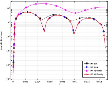
Click Replace Expression in the upper-right corner of the y-Axis Data section. From the menu, choose TBC in the Frequency Domain (comp1) > Thin Layer > Magnetic > mf.normH - Magnetic field norm - A/m.
|
|
5
|
|
6
|
|
7
|
|
1
|
|
2
|
In the Settings window for Point Graph, click Replace Expression in the upper-right corner of the y-Axis Data section. From the menu, choose TBC in the Frequency Domain (comp1) > Thick Layer > Magnetic > mf2.normH - Magnetic field norm - A/m.
|
|
3
|
|
4
|
|
1
|
|
2
|
|
3
|
|
4
|
|
5
|
|
6
|
|
7
|
|
8
|
|
9
|
Click
|
|
1
|
|
2
|
|
3
|
|
4
|
Click Replace Expression in the upper-right corner of the y-Axis Data section. From the menu, choose Fully Resolved Layer in the Frequency Domain (comp2) > Fully Resolved Layer > Magnetic > mf4.normH - Magnetic field norm - A/m.
|
|
5
|
|
6
|
|
7
|
|
1
|
|
2
|
|
3
|
|
4
|
|
5
|
|
7
|
Select the Show legends checkbox.
|
|
8
|
Click to expand the Coloring and Style section. Find the Line style subsection. From the Line list, choose Dashed.
|
|
9
|
|
10
|
|
11
|
|
12
|
|
1
|
|
2
|
|
3
|
|
4
|
|
5
|
Locate the Coloring and Style section. Find the Line style subsection. From the Line list, choose Dashed.
|
|
6
|
|
7
|
|
8
|
|
9
|
|
10
|
|
11
|
Select the Show legends checkbox.
|
|
1
|
|
2
|
|
3
|
|
4
|
|
5
|
|
6
|
|
8
|
|
9
|
|
10
|
|
11
|
|
1
|
|
2
|
|
3
|
|
4
|
|
5
|
|
7
|
Select the Show legends checkbox.
|
|
8
|
Locate the Coloring and Style section. Find the Line markers subsection. From the Marker list, choose Circle.
|
|
9
|
|
10
|
|
11
|
|
1
|
|
2
|
|
3
|
|
4
|
|
1
|
|
2
|
|
3
|
|
4
|
|
5
|
|
1
|
|
2
|
|
3
|
|
4
|
|
5
|
|
6
|
|
1
|
|
2
|
|
3
|
|
4
|
|
5
|
|
6
|
|
1
|
|
2
|
|
3
|
|
4
|
|
5
|
|
1
|
|
2
|
|
3
|
|
4
|
|
5
|
|
6
|
|
7
|
|
1
|
|
2
|
|
3
|
|
4
|
Locate the Plot Settings section.
|
|
5
|
|
6
|
|
1
|
|
2
|
|
3
|
|
1
|
|
2
|
|
3
|
|
1
|
|
2
|
|
3
|
|
1
|
|
2
|
|
3
|
|
1
|
|
2
|
|
3
|
|
1
|
|
2
|
|
3
|
|
1
|
|
2
|
|
3
|
|
1
|
|
2
|
|
3
|