PDF

Submarine Cable 8 — Inductive Effects 3D
Introduction
The previous tutorials in this series — in particular the Capacitive Effects, the Inductive Effects, and the Thermal Effects tutorials — have analyzed the cable in 2D and 2.5D only. Although 2D models have proven to be a very valuable engineering tool, they are fundamentally incapable of capturing the precise, intricate interaction between the phases, the screens, and the armor. The reason for this, is that the phases and the armor are typically twisted with different lay lengths, and in opposite directions (to achieve torsion stability). The same opposite twist, together with the large aspect ratio of the device, tends to turn 3D modeling into a challenge.
In the meantime, computational resources have increased drastically. When investigating research on the matter [2, 7], one cannot help but notice a strong correlation between the year of publishing and the level of detail present in the 3D models. Although advanced solvers, sophisticated mesh configurations and shear computational power have improved the situation a lot over the years, the biggest performance shift is caused by the introduction of twisted periodicity [2] and short-twisted periodicity [3]: Fully detailed 3D cable modeling is now possible within minutes on relatively cheap hardware.
This last tutorial intends to give a “final answer” to 3D cable modeling. It has been developed with feedback from several experts from within the industry, and is on a par with the latest research (2020) when considering both performance and level of detail. Validation is included: The behavior of the models is analyzed within the context of refs. [1, 2, 4, 5, 6, and 7], and the cable’s official specifications.
A Note on Educational Value
Although this tutorial will be of particular use for those working within the cable industry, it is not all “just about cables”. This tutorial — and the entire series, for that matter — is about Electromagnetics, and Numerical Analysis. It is about good engineering practices, about understanding and applying theory, about result validation, and about presenting your results in an attractive and informative way.
The three-phase cable with the magnetic, twisted armor is and ideal device to illustrate and investigate various electromagnetic and numeric phenomena. Since many of these cables are standardized1, their physical properties are available from literature (allowing for validation). At the same time, they are a part of ongoing research. This makes them a suitable tool for industry professionals and academic students alike, to familiarize themselves with the numerical analysis of electromagnetic devices in general.
Model Definition
The 3D geometry represents the same cable as the 2D one used in the previous tutorials (see Figure 1). It has been prepared and discussed in detail, in the Geometry & Mesh 3D tutorial. Apart from being 3D and having a twist, the main difference is that all the insulators have been replaced by one “generic insulator” material (see section Conductors and Insulators). The details that remain, are either necessary because they strongly affect the results (typically the metals), or because they aid meshing and postprocessing. The material properties of the conductors are the same as those used previously.
Figure 1: The cable’s 3D geometry, including the three phases (yellow), screens (red), the XLPE (white), and the armor (blue).
Note: If electromagnetic theory or vector calculus is not your thing, do not worry. Just go to the section Modeling Instructions and you will get there. On the long run however, it is recommended to invest in a deeper understanding of the underlying theory. This will be especially useful during troubleshooting and result interpretation.
Theoretical Basis
The model solves Maxwell–Ampère’s law in the frequency domain, and in 3D, using the magnetic vector potential A as a dependent variable. The theory involved has been treated in full detail in the Theoretical Basis section of the Inductive Effects tutorial. A shortened version is included here. Both texts use the differential form, together with the SI unit system.
When solving, all four Maxwell’s equations are either directly or indirectly involved, together with two field definitions (E and B in terms of A) and three constitutive relations — the ones containing the material properties ε, σ, and μ:
Conservation of Current
Let us start with the conservation of current. When current is not conserved, you get a build-up of charge, as given by ∇ ⋅ J = −jωρ in the frequency domain. You can combine this with Gauss’s law, to get a modified current conservation law:
(1)
Here, the term jωD is known as the displacement current density. As pointed out in the Capacitive Effects tutorial, the displacement current density is prominent in the insulators, the conduction current density is prominent in the conductors, and the sum of both is conserved at all times. This is why some textbooks include the displacement current in the definition of the current density:
(2)
where the two constitutive relations D = εE and J = σE have been used. This relation suggests ωε is some sort of imaginary “conductivity” — one that does not involve losses. It explains why the permittivity can be related to the conductivity in section Conductors and Insulators. It also explains why some people tend to use a complex permittivity in order to model resistive effects in the frequency domain.
Maxwell–Ampère’s law basically states there is a direct relation between the magnetic field H that encircles a conductor and the current density J' that runs through it2. If you take the divergence of that, it results in something very convenient:
(3)
This is true by definition: From basic vector calculus follows that the divergence of the curl of any vector field must always be zero. In other words, if you define the current density to be equal to the curl of H, you get a current conservation law for free — there is no additional equation required to enforce this.
The Magnetic Vector Potential
Gauss’s law and Maxwell–Ampère’s law have now been applied. If you add the third constitutive relation3, B = μ0μrH = μH, you end up with the following:
(4)
Now consider a vector field A, the magnetic vector potential in Vs/m (or Wb/m), whose curl is chosen to be equal to the magnetic flux density B. That is, ∇ × A = B. The magnetic vector potential is not a directly measurable field or anything, nor is it unique. Without any additional constraints there are many different fields A that fulfill the requirement4 ∇ × A = B. Using this relation between A and B, and taking the divergence once again, you get:
(5)
So if you define B in terms of A, you get magnetic flux conservation (Gauss’s law for magnetism) for free. This is for the exact same reason that you got current conservation for free. If you now substitute this definition of B in Maxwell–Faraday’s equation of electromagnetic induction, you get:
(6)
This gives you the last piece of the puzzle5: E = −jωA. Now, both B and E can be expressed in terms of A. If you substitute this result in Equation 4, you will find:
(7)
Finally, if you swap about some terms and put everything on the left-hand side, you get the following 3D partial differential equation for the dependent variable A:
(8)
Due to the double curl, this is known as a curl-curl-type equation. The Magnetic Fields interface uses this equation in the domains to determine the value of A, and consequently, the value of all the fields derived from it: E, D, J, B, and H.
For the outer boundaries the default condition n × A = 0 is used, that constrains A in the direction of the surface normal. Therefore, B will be perpendicular to the surface normal; the magnetic flux lines will flow along the surface. This is known as a magnetic insulation condition (in analogy to electric or thermal insulation). Together with the partial differential equation, the boundary condition gives you a complete set of equations.
In order to excite the system, an external electric field Eext is applied in the cable’s main conductors (for more on this, see section Modeling Instructions). This field comes from an outside source not included in the model, presumably a power plant or a wind farm.
Shape Functions and Discretization Order
In order to solve a partial differential equation like Equation 8 numerically (as opposed to analytically), space needs to be divided into a finite number of elements — hence the term, Finite Element Method (FEM). For this, a mesh is constructed. Each mesh element is associated with a so-called shape function. The “true” solution is then projected onto these shape functions to create a system of equations with a finite number of unknowns, or Degrees of Freedom (DOFs).
The details of this procedure lie outside the scope of this tutorial however6. For now, it is sufficient to consider the shape functions to be the pixels of your digital image. Solving the model amounts to finding the RGB values of your pixels, such that the image approximates the true analogue image as best as possible. What the true analogue image looks like, is described by the partial differential equation.
Pixels in digital images tend to have one single color all over. Shape functions however, can be constant, they can be linear gradients (first order elements), they can be parabolas (second order elements), or even higher order. Second order elements are able to describe the true shape in more detail than linear elements can — much like a higher-order polynomial is better at fitting to a measured dataset. Linear elements however, are much leaner. They describe the solution less accurately, but they are more stable and have less degrees of freedom.
For 2D models, computational resources are rarely an issue. All 2D models in this series use a standard “normal” mesh, with second order elements. For large 3D models however — especially when direct solvers, tricky meshes, and nonlinear materials are involved — the lean and stable properties of first order elements are of crucial importance. The price you pay is less detail, but what you gain is a massive reduction in memory consumption and overall computational effort.
On Numerical Stability
Conductors and Insulators
Electric conductivity is likely to be the material property with the largest range of naturally occurring values (that is; not even considering superconductivity). The cross-linked polyethylene (XLPE) in the cable has an electric conductivity with a value around 1 · 1018 S/m, while the copper has a value of 6 · 107 S/m — a contrast of 6 · 1025. For a finite element model, a contrast of 1 · 106 is already close to what the numerical precision of the system can handle.
In other words, if a device is predominantly inductive (or resistive) and the conductors completely determine the solution, every material with a conductivity several orders of magnitude lower than those can be considered an “insulator”. Likewise, if a device is predominantly capacitive in nature, it will be the insulators determining the solution and any material with a conductivity above 1 S/m can be considered a “conductor” (see the Capacitive Effects tutorial). Accurately capturing both capacitive and resistive effects in the same model at the same time is oftentimes unnecessary and may require an extreme numerical precision.
Admittedly, at higher frequencies this becomes less of an issue, as displacement currents will take over the role of conduction currents in the insulators (that is; Equation 1 will still be solvable). For example, at a frequency of 50 Hz the “total conductivity” of the XLPE can be considered to be σ + jωε, having a norm of ||1018 + 2.5jωε0|| ≈ 7 · 109 S/m. This is already nine orders of magnitude larger than the electric conductivity alone.
Using a Stabilizing Conductivity
The numerical system’s inability to resolve a material contrast much larger than 1 · 106 explains why many electrostatic models will consider metals to be equipotential domains. It also explains why this 3D twisted cable model is working fine with 50 S/m as the conductivity setting for the “generic insulator”. In fact, it needs to have a significantly nonzero value in the insulators. The model would become singular otherwise.
The reason for this can be seen in Equation 8. When the conductivity is too small, the Helmholtz term −ω2εA + jωσA will become numerically insignificant (indistinguishable from zero, given the numerical precision used). This reduces the equation to:
(9)
which is also known as the magnetostatic approximation, that is; all first- and second order time derivatives have been removed from the system of equations. The problem with this, is that it is ungauged (as briefly touched upon in section Theoretical Basis). In other words, Equation 9 does not provide you with enough information to find a unique solution for the magnetic vector potential Ayou can compare this with a linear equation for which you only know the derivatives. For a direct solver, that is a problem.
There are numerous ways around this problem, including different kinds of Gauge Fixing, a mix of different formulations7 (AV-formulation, AVm-formulation), or the use of specialized iterative solvers. One of the most simple and effective tricks in numerical engineering however, is to give the insulators a stabilizing conductivity that is large enough to keep the model numerically stable, yet small enough to not affect the solution significantly.
Note: For inductive devices in the frequency domain, you can use the skin depth to judge whether σ should be considered large or small. When the skin depth is several orders of magnitude larger than the dimension of interest, σ is likely to have no significant influence on the solution. For the insulators with 50 S/m the skin depth evaluates to about 10 m; much larger than the cable’s cross-sectional features.
Finally, notice that this is not an issue for the 2D models, because together with the default boundary condition magnetic insulation, forcing the magnetic vector potential A to be out-of-plane is enough to get a unique solution (as seen in the Inductive Effects tutorial).
Compensated Stabilization
The fourth section of this tutorial — section Modeling Instructions — Compensated Stabilization — discusses an experimental approach that stabilizes the model and subsequently adds a compensation term that mitigates the effects of the stabilization.
Attributing 50 S/m to insulators like air or polyethylene, is much like adding an additional unphysical term to Equation 8:
(10)
This equation is then solved once. “Solving” means, in this case, that the matrix inverse (or LU factorization of it, at least) is determined by the direct solver. The LU factors are then used to determine A. This is how you would normally solve the model.
On several occasions in this tutorial series, the external current density Je is presented as a contributing term, and one that you can consider to be on the right-hand side of Equation 10notice that all terms in this equation represent some kind of current. Adding a contributing term to the right-hand side will not affect the matrix inverse. By setting Je = jω50A, you will arrive at the following:
(11)
If you then solve a second time using the same LU factorization (which should only take a fraction of the time it took initially), the artificial terms on the left- and right-hand side will cancel out and you will have found a new value for the magnetic vector potential: A'. A value that satisfies the original equation, Equation 8.
Looking at it from an engineering perspective; you first introduce a finite conductivity in your insulators, causing a leakage of current Jl = 50E = −jω50A from one conductor to another. You then assess the amount of leakage and install a pump in the insulators that pumps the same amount of current in the opposite direction, affecting the current density distribution in both the insulators and conductors.
The cancellation will not be perfect however8, and the accuracy of the electric fields in the insulators may be affected. The method should not be used when the contrast in material properties is moderate only. In those cases, however, numerical stability is typically not an issue in the first place.
Modeling Approach
The modeling instructions in this tutorial are divided in five sections (as listed below), and for each section a reference file has been saved. This will allow you to start somewhere halfway the tutorial (although going through it from start to finish is recommended).
Extruded 2D Model
The initial goal is just to get a functional model in 3D and get some kind of estimate of the accuracy involved. To this end, the fully parameterized geometry sequence is put into a state where it is essentially no more than a plain extrusion of a 2D geometry. In this state, the 3D geometry should be able to perfectly reproduce the results obtained from the 2D one. That is; if it had the same level of detail of course, and if it were using the same mesh, with the same discretization order.
Comparing the extruded 2D model to the fully detailed plain 2D configuration discussed in the Inductive Effects tutorial, basically allows you to “assess the damage” caused by the concessions you had to make to keep the problem manageable in 3D. The opposite applies too by the way: You will discover the 3D model is amazingly accurate considering the removal of all those details. The topic of accuracy and the relevance of certain details has been discussed several times before, in particular in the Capacitive, Inductive, and Thermal Effects tutorials.
3D Twist Model
After the model has been tested in its extruded 2D state, it will be cranked into “full 3D twist mode” with a twisted periodic condition (see section Twisted Periodicity). This will allow you to investigate the effect of the twist on the magnetic flux-, the current-, and the loss densities in the phases, the screens, and the armor. Furthermore, it allows you to make a comparison with the 2D and 2.5D models (at room temperature). You can validate your comparison further, using sources like reference [2].
Linearized Resistivity 3D
Since this kind of cable normally operates at temperatures around 80–90°C, the material properties of the conductors typically include a temperature correction in the form of linearized resistivity9:
(12)
where ρ0 refers to the reference resistivity at Tref, and α is the resistivity temperature coefficient in 1/K. The models discussed here do not actually solve for T though. Instead, the temperature readings are taken from the fully coupled induction heating model presented in the Thermal Effects tutorial. With the modified material properties, the results are analyzed once again.
Compensated Stabilization
Furthermore, the implementation of the compensated stabilization — as described in section Compensated Stabilization — is demonstrated, and the influence of current leakage between the armor wires on the overall solution is investigated.
The Short-Periodic Configuration
Finally, the geometry and the mesh are modified to allow for a different kind of periodicity, reducing the size of the model a hundredfold while still providing a similar accuracy (see section Short-Twisted Periodicity). The results are compared to the full-periodic model.
On Lay Length and Cross Pitch
The twist adds a new dimension to the device, one that the 2D models cannot capture. The distance required for the phases to complete one full revolution around the cable’s axis, is called the phase’s lay length, or Lpha, see Figure 2. For the armor, a similar reasoning holds. The lay lengths are typically expressed in terms of phase and armor diameter. For the models in this tutorial, we have:
(13)
where Dpha is the outer diameter of all three phases and screens combined, and Darm is the central diameter of the armor wire ring. The minus sign reflects the opposite direction of the armor twist.
The amount of phase and armor twist in degrees per meter length of cable is then given by:
(14)
and the difference in twist angle between the phases and the armor increases with Tpha − Tarm degrees per meter. The amount of meters for which this difference becomes 360°, is what is of interest. This is the length required for the armor to make a full revolution with respect to the phases. At that point, the same armor wire will meet the same phase again, and the pattern will repeat itself (albeit at a different angle, see Figure 3). This length is called the cable’s cross pitch:
(15)
where the degrees cancel out. The long 3D twist models built in this tutorial have a length equal to one times the cable’s cross pitch (although multiple periods are supported).
Figure 2: The cable’s armor lay length and phase lay length (image scaled by a factor of 5 in the longitudinal direction). The lay length is the distance required for the helices to complete a full revolution.
Twisted Periodicity
The tutorial uses a twisted periodicity condition that constrains the magnetic vector potential: Adst = Asrc. When applying this constraint, by default a simple “straight” coordinate transformation is performed, based on the location and orientation of the source and destination planes (consider for example planes that are tilted with respect to each other, as is the case for sector symmetry).
For many cases, this solution works out of the box. The twist will require some further user input though, since the symmetry planes are circular and since the “mismatch” may very well have been intentional — after all, COMSOL supports any kind of geometry, not just those of cables. The orientation of the periodicity plane changes with respect to the global coordinate system as you progress along the cable (see Figure 3, and references [2, 3]). After a distance of CPcab, it has rotated around the cable’s axis, at a twist angle of:
(16)
You may have noticed that, although this expression is based on Lpha, the armor lay length will work just as well: If you compute the twist angle using Larm instead, the value will be negative, and the difference between the two will be one full revolution.
Figure 3: The orientation of the periodicity plane changes as you progress along the cable.
Note: For the twisted periodicity to work properly, it is important that the mesh nodes on the source and destination boundaries coincide. This is because the model uses a vector potential formulation with curl elements in 3D. With a nonconforming mesh the magnetic vector potential will have to be interpolated, causing the accuracy and stability of your model to degrade. The measures you can take to ensure that the mesh is of good quality, are discussed in the Geometry & Mesh 3D tutorial.
In order to add this rotation to the Periodic Condition, you can set a transformation to an intermediate map. Choosing a rotated coordinate system for this map with an Euler angle α equal to Tcp, will apply the appropriate transformation.
Short-Twisted Periodicity
The use of twisted periodicity is based on the observation that the pattern repeats itself as soon as one particular armor wire returns to its original position with respect to a certain phase, regardless of the orientation of the overall cross section. If you look at the results more closely, however, you will see that the pattern repeats itself as soon as any armor wire reaches that particular position — assuming of course, all the armor wires are identical10.
With this knowledge you can configure the periodicity to “connect” each armor wire with its neighbor, rather than itself [3]. The distance it takes for the next armor wire to reach the position that the first one had, is CPcab divided by the number of armor wires: Narm. Especially for cables with a large number of armor wires, this means a massive reduction in model size, both numerically and geometrically; see Figure 4.
The resulting ring of short pieces of armor wire can either be seen as a slice of the actual cable, or a number of small sections of armor wire that are connected in series to form one full-periodic armor wire: The two descriptions are equivalent.
Figure 4: The mesh in the armor rotates clockwise, while the remaining mesh rotates counterclockwise. The source periodicity plane is at the bottom, and the destination is at the top.
Short-Twisted Periodicity and Mesh Conformity
The short-twisted periodicity does not come entirely for free, however: The meshing procedure will require some additional attention. If the meshes are to be equal on the two periodicity planes — to get conforming meshes, see the Geometry & Mesh 3D tutorial — the cross-sectional mesh of each of the armor wires will need to be identical. After all, the short-twisted periodicity causes the armor wires to switch places when going from the source plane to the destination plane.
Consider Figure 4 once again: The ring that contains the armor wires has a clockwise twist, while the rest of the mesh rotates counterclockwise. After a distance of CPcab/Narm, the cross section will look the same — albeit twisted at an angle of Tcp/Narm, and with the armor wires having switched one position. For the domains indicated in yellow a swept mesh will be used and mesh conformity will follow naturally there. For the gray surfaces, special care needs to be taken to make sure that the mesh on the destination plane is rotated to the same degree — and in the same direction — as the mesh in the phases.
In practice, this means that the circle that marks the outer perimeter of the model should be part of the work plane Phases and Screens (wp1). The part of the periodicity plane that is exterior to the cable and the part in-between the screens and the armor, will have to be copied from the source to the destination using a Copy Face operation. Additionally, the mesh in and around the armor wires will have to be modified to ensure that the mesh is the same for each one of them.
Short-Twisted Periodicity and Double-Twisted Armors
For a single helix, “straight” periodicity requires a model as long as the lay length — but twisted periodicity supports any length. For a double helix with separate lay lengths, “straight” periodicity requires the least common multiple of the two lay lengths (which may be over 40 meters) — but twisted periodicity only requires a length equal to CPcab (which is about 1.6 m in our case). Now, using short-twisted periodicity you can reduce this even further, to a mere 1.5 cm (assuming 110 identical armor wires).  
So, what happens if you add a double-twisted armor?
For the double armor, you will have to search for the least common multiple once more. The main difference is that with short-twisted periodicity, the distances involved are much smaller. Also, assuming the armor wires are identical, you may choose which wires to connect (the nearest neighbor, the second neighbor… and so on).
Consider a short-periodic model having a length CPcab/Narm = Lsp, and a secondary armor with a number of armor wires, equal to Narm2. The secondary armor will definitely fit if it has the same twist as the phases: Tcp/Narm. Other valid values are:
(17)
where n is an integer {2, 1, 0, +1, +2, …} indicating how many places the wires have switched position. If you do not find a value that is close enough to reproduce your desired cable geometry, you can simply go to the next periodicity plane, at a distance of 2Lsp, or one of the planes after that: mLsp (where m is another integer). The secondary armor’s lay length is then given by:
(18)
In the table below, this lay length (in meters) is shown as a function of n and m. Here, the values for Lsp and Lpha are the same as before, and Narm2 is chosen to be 119. For larger values of m, it will be easier to find a value of n that fits your needs. In order to keep the computational effort low, you can allow for a variation of “±5 cm” on the lay lengths involved and solve an optimization problem that minimizes the error on all of them for a given value of (n, m). And when in doubt, just test a couple of different lay lengths to see if it makes a difference in the first place.
Results and Discussion
Extruded 2D Model
The extruded 2D model behaves very much like an ordinary 2D model. The magnetic flux is contained almost entirely in the xy-plane, and the currents point in the z direction only. This does not mean the agreement with the plain 2D configuration presented in the Inductive Effects tutorial is perfect, however. Two error estimations have been obtained: One by looking at the transverse current density norm (that is supposed to be zero), and another by comparing the results with those from the 2D models.
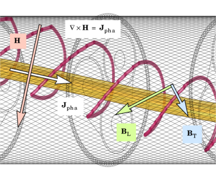
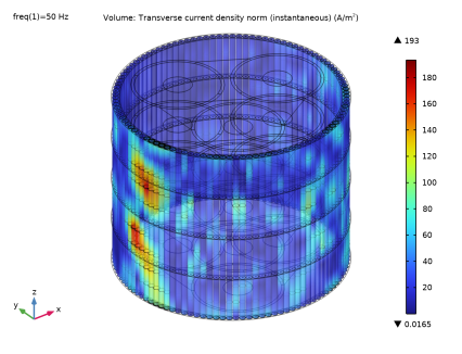
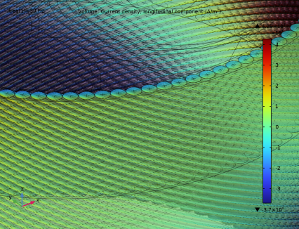
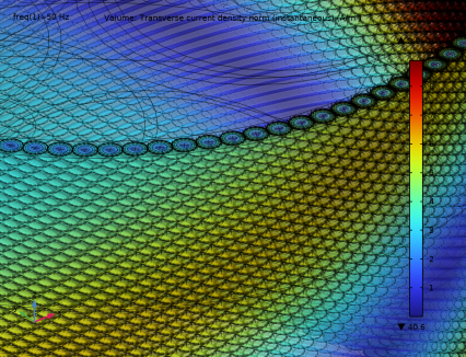
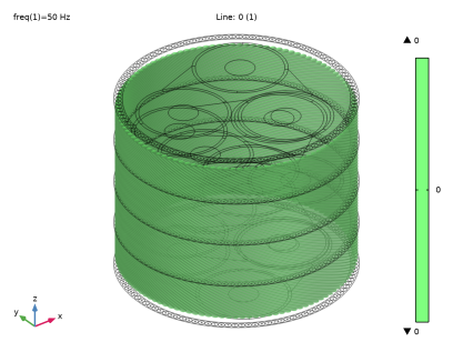
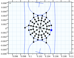
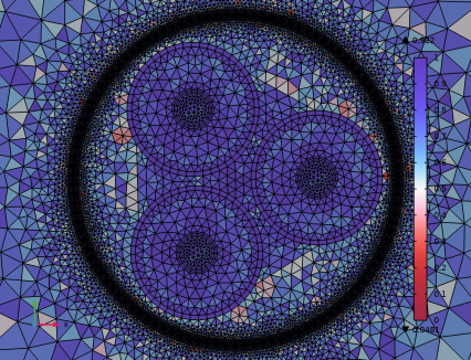
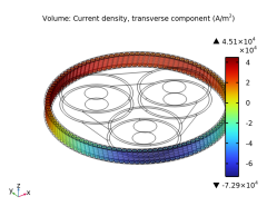
The transverse current density norm is noisy with a maximum around 100–200 A/m2. This is about 2000 times less than the maximum norm of the longitudinal current density abs(mf.Jz), and can be seen as an attempt of the numerical system to approximate “zero”. In other words, a reasonable guess for the margin of error in the armor currents is 100–200 A/m2.
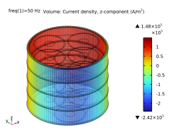
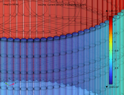
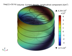
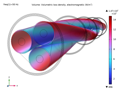
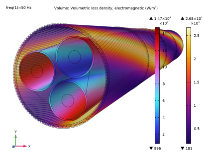
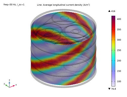
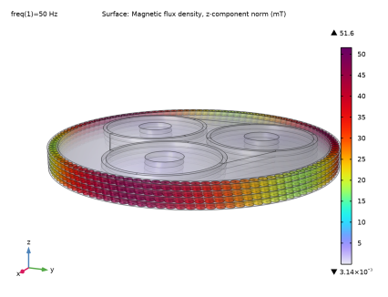
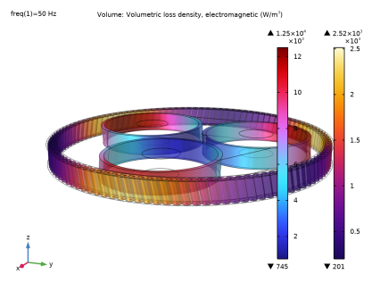
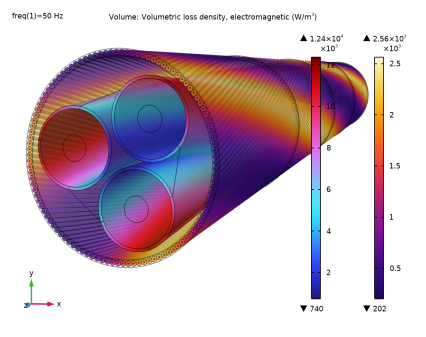
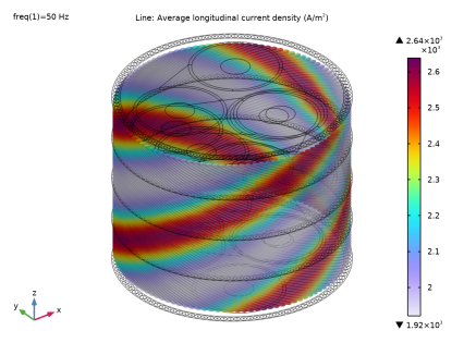
The losses are about 47 kW, 12.6 kW, and 7.4 kW per kilometer for the phases, screens, and armor respectively. The AC resistance is about 52 mΩ/km and the inductance is 0.41 mH/km. The overall deviation with respect to a fully detailed 2D model seems to lie around 0.5–1%.
All numbers are slightly lower than those from the 2D model. The primary cause of this seems to be the coarse mesh together with the lower element order, making the problem stiffer — and not the use of polygons instead of circles, the removal of geometrical details in the insulators, or the use of a stabilizing conductivity.
You can verify this statement quite easily, by building 2D models with various levels of detail, testing different mesh sizes and discretization orders, and comparing the results with both the detailed 2D models and the extruded 2D model from this series.
3D Twist Model
In the 3D twist model, the magnetic flux density in the armor develops a large longitudinal component. In fact, the flux is primarily in the longitudinal direction here, see Figure 5. The magnetic field encircles the phase currents, as given by Ampère’s law ∇ × H = Jpha. At the same time, the magnetic flux density B will try to find the path of least reluctance.
Since the armor is a good magnetic conductor, the flux lines will quickly find their way to the armor [2, 6]. This is true for both 2D models and 3D twist models.
Figure 5: The norm of the longitudinal magnetic flux density component.
Figure 6: The magnetic field H encircles the phase conductor. Having arrived at the armor, the flux can choose between a longitudinal direction BL, or a transverse one BT.
Once the flux lines get there however, things will be different. In a 2D model, the only option for the flux to complete its loop, is to hop from one armor wire to another. For the 3D case, the opposing twist allows for an alternative route: The flux lines enter the armor, follow the armor wires for a short distance, and then return to the cable center where they circle around the phase conductor (see Figure 6). The resulting path is a helix rather than a straight loop, so at the end of the cable the flux will have to exit on one side of the cross section and reenter on the other.
Plotting either the longitudinal or transverse component of the magnetic flux in the armor shows that both options — hopping between the wires, and following the wires — coexist. The ratio between the two, is governed by the reluctance of the involved paths. Increasing the gap between the wires will benefit the longitudinal flux, and increasing the cable’s cross pitch (or decreasing the armor’s permeability) will benefit the transverse flux.
The longitudinal flux BL in the armor wires is linked to a transverse current density JT, through Faraday’s law of electromagnetic induction ∇ × ET = −jωBL. Likewise, the transverse flux BT is linked to a longitudinal current density JL. The transverse currents form small eddies that circle within the wire’s cross section. Their norm has a cone shape, as shown in Figure 7.
Figure 7: The transverse currents form eddies in the cross section of the wire (the cones), the longitudinal currents flow back and forth and are zero on average (the gradients). An animated version is available as reference [9].
The longitudinal currents move back and forth in the wire, and are about zero when integrated over the wire’s cross section. This is because 1) the armor wires spiral around the phase conductors, and 2) because the cable is well-balanced. The combination of these two makes the total net electromotive force (emf) that the wires are subjected to, zero.
Locally however, the closest phase is able to push the currents forward on the inside of the armor, making them flow back on the outside. If the cable would lose balance, the net armor wire current would deviate from zero, but should still have the same value for all wires (because of symmetry reasons). It is this logic that is the basis for the 2.5D models — where the armor wires have been connected in series [7]. Unsurprisingly, the longitudinal currents strongly resemble those produced by a 2.5D model.
Comparison between 3D, 2D, and 2.5D
The comparison is shown in Table 2. Although the balance between phase, screen, and armor loss differs between 2D and 3D, the total loss is surprisingly similar. The same goes for the AC resistance11.
The relatively high loss values given by the plain 2D model — as compared to 2.5D (with or without milliken phase conductors) — is caused by the unconstrained armor currents. The 3D twist losses are higher than the 2.5D ones too, but there the cause seems to be the transverse eddies, the strong increase in magnetic hysteresis losses in the armor, and the lower overall reluctance of the magnetic circuit.
In 3D the armor wires are twisted, giving the flux an alternative, low-reluctance path. Furthermore, the twist shortens the cable and compresses the armor wires, reducing the space between them. Notice that the spacing between the wires in the 2D models is actually an over-estimation. These effects cause the armor to behave more like a magnetic core: The fields are confined more to the interior of the cable where the phases and screens are. Consequently, both the inductance and the AC resistance increase.
So one may argue that the plain 2D configuration gives the “right” resistance for the “wrong” reasons, and that this may be an issue for academic applications. As an engineering solution however, the 2D model is still a perfectly legitimate tool12.
The 2.5D model correctly reduces the longitudinal currents, but fails to include the other effects caused by the twist (hence, the underestimated AC resistance). The large value for the inductance seems to be “spot on” compared to the 3D model, but is not caused by the same effects. As it turns out, suppressing induced currents decreases reluctance as well — just as a higher permeability or a thinner air gap would (this effect will show up once more when adding linearized resistivity). So here too, you can argue that it gives the “right” value for the “wrong” reasons.
Exactly how the 2D, 2.5D, and 3D models relate to each other and to measurements (and what margins of error may be expected), has been further investigated in reference [2]. In practice, 3D models would typically be used by cable manufacturers and academics who feel the need to get a good understanding of the physics involved (or to validate their 2D models). 2D and 2.5D models may be more suitable for end users of cable systems who intend to investigate whether their cable duct provides adequate cooling, for example.
Figure 8: The volumetric loss density in the armor and screens, for the case where a first-order temperature correction has been applied.
Linearized Resistivity 3D
The default material properties used in the 3D twist model have all been measured at room temperature. Because these cables typically operate at temperatures around 80–90°C, adding a first-order temperature correction basically means increasing the resistivity in all conductors by about 20–30%. As a consequence, the loss balance in the active (current driven) and passive (voltage driven) conductors will change. The effects are similar to those seen in the 2D induction heating models from the Inductive Effects tutorial, see Table 3.
The phase losses go up, but not as much as you would expect, based on Equation 12, and the relation Q = I2R. This is because the phases carry both applied and induced currents. For the applied currents, the stationary-electric I2Rdc-reasoning will hold, but for the voltage driven induced currents, it will not. For those, a V2/Rdc-reasoning should be applied instead — that is; if one still wants to look at it from a static perspective at all13.
As opposed to the phases the screens carry induced currents only, so one would expect losses to go down. They do, but not as much as you would expect based on stationary-electric reasoning (see Figure 8). This is because the reduced induced phase currents are now less effective in screening the fields coming from the applied phase currents. So the lead sheath will perceive a stronger emf coming from the phases. For the armor, there is yet another complication; the resistive losses decrease, but the lack of screening causes the magnetic hysteresis losses to increase even further (to about 75% of the total armor loss).
When the resulting losses are fed back into a 2D thermal model, the temperatures that result are slightly different. Those can then be put back into the 3D model, to apply a second-order temperature correction. This correction term is negligible compared to the first one though (the total losses go up by about 100–200 W/km), and would typically not be considered “worth the effort”. On the other hand, the quick convergence of these correction terms does have a nice implication: It would allow for a hybrid 2D/3D fully coupled induction heating model.
Compensated Stabilization
As part of the demonstration of compensated stabilization, the average longitudinal current density in the armor has been evaluated for each wire individually (by integrating over the wire’s cross section, see Figure 9). These net currents are an order of magnitude smaller than the overall longitudinal and transverse current densities (Figure 7), but they are not zero. They use the finite conductivity between the armor wires to hop from one wire to another, and follow the path they would have taken if the armor were a solid tube.
Figure 9: The average longitudinal current density in the armor, before applying the compensation term.
The first-order correction applied by the stabilization compensation (see section Compensated Stabilization) reduces these currents by a factor of 6: To a level that is about twice as high as the margin of error established in section Extruded 2D Model.
The overall loss in the insulators is reduced by a factor of 600–700 (from 0.1 kW/km to 0.0002 kW/km), but all the other figures stay more or less the same. Apart from the insulator losses, the most significant change seems to be in the AC resistance (somewhere in the 3rd significant digit or so)14. The compensation term works as intended, but at the same time it shows there is not much to compensate for. That is; this confirms once more that the use of a stabilizing conductivity is a very effective and totally legitimate method.
As such, this model is not a demonstration of a case where the compensation term is really needed. Rather, it serves as a proof of concept (POC). This phenomenon is not restricted to cables. The same strategy can be implemented for cases where the effect of the finite insulator conductivity is more significant. Its effectiveness and accuracy may differ between models though, so validation will remain important.
The Short-Twisted Configuration
Assuming the armor wires are indistinguishable, the short-twisted configuration should produce the exact same results as the model that uses the “standard” twisted periodicity. An evaluation of the phase-, screen-, and armor losses, the phase AC resistance and the phase inductance, shows this is indeed the case.
Overall the results deviate by about 0.1–0.4%, but for the armor the difference is a bit larger; about 1–2%. This does not come as a complete surprise though, as the mesh used for the short-periodic armor is much finer than its long-periodic counterpart.
On Magnetic Material Properties
When modeling electromagnetic devices, one of the trickier parts is obtaining reliable material properties for your magnetic components. The problem is that the constitutive relation for B and H is often nonlinear and temperature dependent, and will differ between steel grades and even between individual batches [4, 5]. Even dropping your sample after performing the measurement may be enough to render your measurement inaccurate.
In practice you can either rely on your own measurements, rely on the data provided by your steel supplier, or try to make a good estimate based on material data available in the literature — preferably a combination of all three. Regardless, you should take your material data with a grain of salt.
Please keep in mind though, that even if the material data is off by 10%, the numerical model may still show very accurate overall behavior. For example, the 3D twist model included here shows that the overall inductance of the cable will increase:
The model predicts that if you create a good magnetic connection between your armor wires (using a thin gap and a large contact surface), the losses in your cable will go up drastically. Likewise, the addition of polyethylene (PE) spacer rods between the armor wires is expected to lead to an improvement (from an electromagnetic viewpoint at least). These kinds of observations make the model useful regardless whether you have access to accurate input data.
Generally speaking however, it is always good to validate your models and combine them with measurements and findings from literature.
References
1. International Electrotechnical Commission, Electric cables – Calculation of the Current Rating; IEC 60287; IEC Press: Geneva, Switzerland, 2006.
2. J.C. del-Pino-López, M. Hatlo, and P. Cruz-Romero, “On Simplified 3D Finite Element Simulations of Three-Core Armored Power Cables,” Energies 2018, 11, 3081.
3. D. de Vries, “3D Cable Modeling in COMSOL Multiphysics®IEEE Spectrum, 2020.
4. M. Hatlo, E. Olsen, R. Stølan, and J. Karlstrand, “Accurate Analytic Formula for Calculation of Losses in Three-Core Submarine Cables,” Proc. 9th Int’l Conf. on Insulated Power Cables (Jicable’15).
5. M.M. Hatlo, and J.J. Bremnes, “Current Dependent Armour Loss in Three-Core Cables: Comparison of FEA Results and Measurements,” (Cigré 2014).
6. D. Willen, C. Thidemann, O. Thyrvin, D. Winkel, and V.M.R. Zermeno, “Fast Modelling of Armour Losses in 3D Validated by Measurements,” Proc. 10th Int’l Conf. on Insulated Power Cables (Jicable’19).
7. J.J. Bremnes, G. Evenset, R. Stølan, “Power Loss and Inductance of Steel Armoured Multi-Core Cables: Comparison of IEC Values with 2.5D FEA Results and Measurements,” (Cigré 2010).
8. J.M. Jin, The Finite Element Method in Electromagnetics, 3rd Edition, Wiley, 2014.
9. Video file submarine_cable_z_animation_08_3d_armor_currents, available for download at www.comsol.com/model/cable-tutorial-series-43431.
Application Library path: ACDC_Module/Tutorials,_Cables/submarine_cable_08_inductive_effects_3d
Modeling Instructions
This tutorial will focus on inductive effects in 3D, both at room temperature and at elevated temperatures. The instructions on the following pages will help you to build, configure, solve and analyze the models. They are organized in five sections:
Modeling Instructions (including Modeling Instructions Extruded 2D Model).
These sections represent the five stages, as described in section Modeling Approach. In-between these sections the model is saved and reopened. This will allow you to get back on track when you made a mistake, or to skip parts on purpose — although going through the instructions from start to finish is recommended.
If anything seems out of order, please retrace your steps. The reference files — available in the model’s Application Libraries folder — can help you out. You can compare them directly to your current model by means of the Compare option in the Developer toolbar. When doing so however, remember that some settings stored in your model may depend on your operating system, COMSOL version or COMSOL Desktop configuration: There will likely be some deviation from the reference files.
A Note on Geometry Handling and Meshing
The camera setup, geometry sequence, selections and mesh have been prepared in the file submarine_cable_07_geom_mesh_3d.mph. This file results from the previous tutorial in this series. Although the physics typically gets most attention in publications and marketing material, it should be pointed out that the geometry handling and meshing oftentimes represents a major part of the efforts spent on a large 3D FEM model such as this one. It is therefore recommended to have a look at the Geometry & Mesh 3D tutorial first (if you have not already done so).
Root
Either way, you can start this tutorial by opening the prepared file and saving it under a new name.
1
From the File menu, choose Open.
2
3
From the File menu, choose Save As.
4
Browse to a suitable folder and type the filename submarine_cable_08_a_inductive_effects_3d.mph.
Global Definitions
The model contains a parameter called Nper. This parameter sets the number of cable cross pitch periods CPcab included in the model, by making the geometry longer or shorter (for more on this, see section On Lay Length and Cross Pitch). We will set its value to 1/10 shortly. This will shorten the geometry by a factor of ten. Furthermore, since Nper will not be integer any longer, there will be no periodicity as long as a twist is present. The parameter Tenab will turn “0” (false), disabling the twist and turning the geometry into a plain extrusion.
Hint: If you press Ctrl+F and search for the string “Nper” in the model, you can see where it has an effect.
As this reduces the solving time from half an hour to one minute or so, it will allow you to quickly configure and test your model before going full scale — which is generally considered to be a good modeling practice. Additionally, it will allow you to investigate how well the 3D model coincides with the plain 2D configuration discussed in the Inductive Effects tutorial. Theoretically there should be no difference, but numerically, there will be.
Geometric Parameters 3
1
In the Model Builder window, under Global Definitions click Geometric Parameters 3.
2
In the Settings window for Parameters, locate the Parameters section.
3
Electromagnetic Parameters
1
In the Model Builder window, click Electromagnetic Parameters.
2
In the Settings window for Parameters, locate the Parameters section.
The electromagnetic parameters are the same as those used in the Inductive Effects and Capacitive Effects tutorials. They have already been loaded in the Geometry & Mesh 3D tutorial, because the boundary layer mesh depends on the skin depth.
The parameters f0 (w0), V0 and I0 are the operating frequency, the phase to ground voltage and the rated current respectively. The factors 1/sqrt(3) and sqrt(2) convert from phase-to-phase to phase-to-ground, and from root mean square (RMS) to peak value. The other parameters are related to material properties and analytical descriptions of the cable.
Now that Nper has been set, it is time to rebuild the geometry. Proceed by switching views.
Geometry 1
1
In the Model Builder window, expand the Component 1 (comp1) node, then click Geometry 1.
2
Click the Go to View 1 (Orthographic) button in the Graphics toolbar.
At first the cable looks stretched, because the camera is using the latest parameter values while the geometry has not yet been rebuilt.
3
In the Geometry toolbar, click  Build All.
The result is a cable section of only 16 cm long, without twist. This will be the geometry used for small scale testing.
Next, let us have a look at the physics. Start by adding a Magnetic Fields interface.
Add Physics
1
In the Home toolbar, click  Add Physics to open the Add Physics window.
2
Go to the Add Physics window.
3
In the tree, select AC/DC > Electromagnetic Fields > Magnetic Fields (mf).
4
Click the Add to Component 1 button in the window toolbar.
5
In the Home toolbar, click  Add Physics to close the Add Physics window.
Magnetic Fields (mf)
Free Space 1
For the electromagnetic analysis, the default domain condition is Free Space; it models air, vacuum, or a “generic insulator”. You can consider it the empty canvas to draw on.
It comes with a built-in stabilization option. We will choose a stabilization conductivity that corresponds to a skin depth of six times the typical length scale of the model: about 50[S/m]. Why that is, and whether the chosen value should be considered large or small (and how its value has been determined in the first place), is part of an important discussion — see section On Numerical Stability. In addition to this, an experimental approach that helps you to mitigate the effects of the finite conductivity is presented in section Modeling Instructions — Compensated Stabilization.
1
In the Settings window for Free Space, locate the Stabilization section.
2
From the σstab list, choose From skin depth.
3
Find the Skin depth subsection. In the δs text field, type 6*CPcab.
Next, in order to model solid domains, add an Ampère’s Law in Solids feature.
Ampère’s Law in Solids 1
1
In the Physics toolbar, click  Domains and choose Ampère’s Law in Solids.
2
In the Settings window for Ampère’s Law in Solids, locate the Domain Selection section.
3
From the Selection list, choose Conductors.
To solve the model, prepare a Frequency Domain study, and a Coil Geometry Analysis study step.
Add Study
1
In the Home toolbar, click  Add Study to open the Add Study window.
2
Go to the Add Study window.
3
Find the Studies subsection. In the Select Study tree, select General Studies > Frequency Domain.
4
5
In the Home toolbar, click  Add Study to close the Add Study window.
Study 1
Step 1: Frequency Domain
1
In the Settings window for Frequency Domain, locate the Study Settings section.
2
In the Frequencies text field, type f0.
Step 2: Coil Geometry Analysis
1
In the Study toolbar, click  More Study Steps and choose Other > Coil Geometry Analysis.
As the Coil Geometry Analysis is a preprocessing step, it needs to be executed before the frequency domain analysis:
2
Right-click Step 2: Coil Geometry Analysis and choose Move Up.
Materials
The materials are roughly the same as those used in the Inductive Effects tutorial. First, the materials will be added, they will be given an appropriate label, a selection and an appearance. Then, we will fill in their properties.
Copper
1
In the Model Builder window, under Component 1 (comp1) right-click Materials and choose Blank Material.
2
In the Settings window for Material, type Copper in the Label text field.
3
Locate the Geometric Entity Selection section. From the Selection list, choose Phases.
4
Click the Zoom to Selection button in the Graphics toolbar.
5
Click to expand the Appearance section. From the Material type list, choose Copper.
Lead
1
Right-click Materials and choose Blank Material.
2
In the Settings window for Material, type Lead in the Label text field.
3
Locate the Geometric Entity Selection section. From the Selection list, choose Screens.
4
Click to expand the Appearance section. From the Material type list, choose Lead.
Galvanized steel
1
Right-click Materials and choose Blank Material.
2
In the Settings window for Material, type Galvanized steel in the Label text field.
3
Locate the Geometric Entity Selection section. From the Selection list, choose Cable Armor.
4
Click to expand the Appearance section. From the Material type list, choose Steel.
Materials
Now, you will see that COMSOL starts detecting missing material properties. The properties that should be added are listed in the following table. Please check all of them for the correct value, even the ones that are already filled in. Note that for cases like this, a convenient option is to copy-paste the values directly from this *.pdf file to COMSOL.
1
In the Model Builder window, under Component 1 (comp1) > Materials, add the following material properties:
Another thing that might have your interest is the relative permeability of the armor: Marm. The chosen value of 100 50j (as defined in Electromagnetic Parameters) has been taken from reference [2], and further verified using [4, 5]. However, the same sources will tell you the permeability will depend on the magnetic field strength and the temperature, and will vary between steel grades (even from batch to batch). Choosing the “right” value for Marm is therefore not trivial, see section On Magnetic Material Properties.
Finally, there is the expression for the copper conductivity. Here, Ncon is the ratio between the copper’s true cross sectional surface area Acon, and the phase cross section used in the geometry: pi*(Dcon/2)^2. This ratio is below unity since the phases are not actually solid, but consist of a bundle of compacted strands with some insulation or gaps in-between (for more on this, see the Inductive Effects tutorial).
Modeling Instructions — Extruded 2D Model
With the materials set and double-checked, it is time to have another look at the physics. The first step in this tutorial is to build a simple extruded model, equivalent to the plain 2D configuration presented in the Inductive Effects tutorial. For this, all you really need are three Coil features (on top of the default Ampère’s Law feature). Although a Periodic Condition is strictly speaking not necessary at this point — that is; Magnetic Insulation should suffice — it is good to have that included too (in preparation for the twist model).
Finally, please remember this tutorial completely neglects the capacitive effects between the phases (the 127 kV phase-to-ground voltage is not considered here). Why this is and whether this is a valid approach, is discussed in the Capacitive Effects tutorial.
Magnetic Fields (mf)
Start by setting the discretization for the magnetic vector potential to linear. For more on this, see section Shape Functions and Discretization Order.
1
In the Model Builder window, under Component 1 (comp1) click Magnetic Fields (mf).
2
In the Settings window for Magnetic Fields, click to expand the Discretization section.
3
From the Magnetic vector potential list, choose Linear.
Periodic Condition 1
1
In the Physics toolbar, click  Boundaries and choose Periodic Condition.
2
In the Settings window for Periodic Condition, locate the Boundary Selection section.
3
From the Selection list, choose Cross Section, Top and Bottom.
4
Click the  Zoom to Selection button in the Graphics toolbar.
The periodicity is oriented in the z direction; it connects top and bottom. At this point it represents a very simple mapping from z = Lsec/2, to z = +Lsec/2. When the twist is added in the next section, things will get more interesting.
Phase 1
1
In the Physics toolbar, click  Domains and choose Domain Coil.
2
In the Settings window for Domain Coil, type Phase 1 in the Label text field.
3
Locate the Domain Selection section. From the Selection list, choose Phase 1.
Switch views and disable the orthographic projection temporarily, to get a good look at the coil domain-, coil input-, and coil output selections.
4
In the Graphics window toolbar, clicknext to  Go to Default View, then choose Go to View 2 (Orthographic, Top).
5
Click the  Wireframe Rendering button in the Graphics toolbar once (to turn it on).
6
Click the  Orthographic Projection button in the Graphics toolbar once (to turn it off).
The settings window for the coil feature contains a lot of sections. For many of these, the default settings are sufficient. Collapse them to have a closer look at the important part; the Coil section.
7
Click to collapse the Material Type section, the Coordinate System Selection section, and the Constitutive Relation sections.
Next, proceed by setting the coil current and the input- and output selections.
8
Locate the Coil section. In the Icoil text field, type I0.
Input 1
1
In the Model Builder window, expand the Component 1 (comp1) > Magnetic Fields (mf) > Phase 1 > Geometry Analysis 1 node, then click Input 1.
2
In the Settings window for Input, locate the Boundary Selection section.
3
From the Selection list, choose Cross Section, Top.
Notice that the selection that is being used, is actually the intersection of “what is chosen” (Cross Section, Top) and “what is applicable” (Phase 1, Exterior Boundaries). You can use this behavior to your advantage. For example, when you start duplicating this coil domain in order to create Phase 2 and Phase 3, you will see the input and output selections for those will follow naturally from the domain selection used in the coil feature. For more on selections, see the Geometry & Mesh 3D tutorial.
Output 1
1
In the Physics toolbar, click  Attributes and choose Output.
2
In the Settings window for Output, locate the Boundary Selection section.
3
From the Selection list, choose Cross Section, Bottom.
In essence, the Input and Output boundary selections are used in a simple diffusion problem, solved by the Coil Geometry Analysis study step (mathematically equivalent to electrostatics or stationary electric currents). This diffusion problem will then provide you with the external electric field distribution Eext needed to excite the currents in the Frequency Domain study step.
In the frequency domain, the total electric field will be the sum of this external electric field and the induced electric field — that is; the electric field caused by electromagnetic induction: jωB, or dB/dt. The strength of the external field will be chosen such that the total net current density integrated over the phase’s cross section matches the current that you have specified: I0.
Note that the coil feature with conductor model Homogenized multiturn behaves differently in this regard (see the Inductive Effects and Thermal Effects tutorials). Let us proceed by duplicating the first phase.
Phase 2
1
In the Model Builder window, right-click Phase 1 and choose Duplicate.
2
In the Settings window for Domain Coil, type Phase 2 in the Label text field.
3
Locate the Domain Selection section. From the Selection list, choose Phase 2.
4
Locate the Coil section. In the Icoil text field, type I0*exp(-120[deg]*j).
Feel free to check if the input and output selections worked out correctly:
Input 1
1
In the Model Builder window, expand the Component 1 (comp1) > Magnetic Fields (mf) > Phase 2 > Geometry Analysis 1 node, then click Input 1.
2
In the Graphics window, check the Boundary Selection.
Output 1
1
In the Model Builder window, click Output 1.
2
In the Graphics window, check the Boundary Selection.
Phase 3
1
In the Model Builder window, right-click Phase 2 and choose Duplicate.
2
In the Settings window for Domain Coil, type Phase 3 in the Label text field.
3
Locate the Domain Selection section. From the Selection list, choose Phase 3.
Re-enable the orthographic projection to restore the camera to its original state. This turns out to be convenient when the geometry gets more complicated later on.
4
Click the  Orthographic Projection button in the Graphics toolbar.
5
Click the  Wireframe Rendering button in the Graphics toolbar.
6
Locate the Coil section. In the Icoil text field, type I0*exp(+120[deg]*j).
Note that, since we are in the frequency domain, expressions like exp(+120[deg]*j) or exp(-j*2*pi/3) may be used to set a 120° phase shift between the AC currents in the three main conductors.
With three coil features to excite your model and Ampère’s law everywhere else (with default settings applied), you should be free to go. Solving this model on a modern desktop machine should only take a minute and consume about 8 GB of RAM. At this point it has about 330 thousand degrees of freedom, or 0.3 MDOF.
Please make sure though, you have a Coil Geometry Analysis study step first, a Frequency Domain study step second, and the frequency set to f0. Proceed by disabling the default plots and computing the solution.
Study 1
1
In the Model Builder window, click Study 1.
2
In the Settings window for Study, locate the Study Settings section.
3
Clear the Generate default plots checkbox.
4
In the Study toolbar, click  Compute.
After COMSOL has finished solving, add a simple plot to get a first impression of your solution.
Results
Magnetic Flux Density Norm (mf)
1
In the Results toolbar, click  3D Plot Group.
2
In the Settings window for 3D Plot Group, type Magnetic Flux Density Norm (mf) in the Label text field.
Multislice 1
1
In the Magnetic Flux Density Norm (mf) toolbar, click  More Plots and choose Multislice.
2
The default plot settings are not that bad. The plot is informative, but it does look a bit boring.
In publications and presentations it is quite common to use default settings like this, because creating aesthetically pleasing yet informative illustrations is not that easy (and oftentimes, is not given priority). However, if you want to impress your superiors and customers with your work — or want your publications to stand out from the crowd — appearance is important.
The next few pages will be about creating fancy yet informative plots using some of the many postprocessing tools that COMSOL provides. After that, we will have a look at the losses, resistance and inductance, and compare them with those from the plain 2D model. To start with, you can exclude the sea bed from the plots by adding a selection to the solution.
Study 1/Solution 1 (sol1)
In the Model Builder window, expand the Results > Datasets node, then click Study 1/Solution 1 (sol1).
Selection
1
In the Results toolbar, click  Attributes and choose Selection.
2
In the Settings window for Selection, locate the Geometric Entity Selection section.
3
From the Geometric entity level list, choose Domain.
4
From the Selection list, choose Cable Domains.
5
In the Graphics window toolbar, clicknext to  Go to Default View, then choose Go to View 5 (Perspective).
If you have not seen the previous tutorial, you might be surprised the cable looks about ten times longer as it did in the other views. The reason for this is that this camera uses a different scaling. For more details on the camera settings, see section Modeling Instructions Camera Setup in the Geometry & Mesh 3D tutorial.
The cable geometry is anisotropic with a clear cross section and longitudinal direction, and a plot of the cross section will capture a large part of the relevant physics (which is why the 2D models work). When a twist is added to the geometry, the cross section will vary along the cable (see Figure 3). To this end, it is very useful to have a plot that shows multiple cross sections in a 3D context.
Cut Plane 3
1
In the Results toolbar, click  Cut Plane.
2
In the Settings window for Cut Plane, locate the Plane Data section.
3
From the Plane list, choose xy-planes.
4
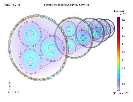
Select the Additional parallel planes checkbox.
5
In the Distances text field, type Lsec*{-1/2,-1/4,1/4,1/2}.
6
Magnetic Flux Density Norm (mf)
1
In the Model Builder window, under Results click Magnetic Flux Density Norm (mf).
2
In the Settings window for 3D Plot Group, locate the Data section.
3
From the Dataset list, choose Cut Plane 3.
4
Locate the Plot Settings section. From the View list, choose View 5 (Perspective).
5
Locate the Color Legend section. Select the Show maximum and minimum values checkbox.
You will not need the multislice plot this time. Remove it to make room for the surface plot:
Multislice 1
In the Model Builder window, right-click Multislice 1 and choose Delete.
Surface 1
1
Right-click Magnetic Flux Density Norm (mf) and choose Surface.
2
In the Settings window for Surface, locate the Coloring and Style section.
3
From the Color table list, choose Prism.
4
From the Color table transformation list, choose Nonlinear.
5
Set the Color calibration parameter value to -0.8.
6
In the Magnetic Flux Density Norm (mf) toolbar, click  Plot.
As there is no twist yet, all cross sections look the same.
In order to show how the conductors twist around the axis, you can add a volume plot based directly on Study 1/Solution 1 (sol1). In this case we apply a selection that includes all conductors, but if you wish to have a better look at the cross sections you can choose a subset of the conductors as well (as done in Figure 2 and Figure 3, for example).
Volume 1
1
Right-click Magnetic Flux Density Norm (mf) and choose Volume.
2
In the Settings window for Volume, locate the Data section.
3
From the Dataset list, choose Study 1/Solution 1 (sol1).
4
Click to expand the Title section. From the Title type list, choose None.
5
Click to expand the Inherit Style section. From the Plot list, choose Surface 1.
Selection 1
1
Right-click Volume 1 and choose Selection.
2
In the Settings window for Selection, locate the Selection section.
3
From the Selection list, choose Conductors.
4
In the Magnetic Flux Density Norm (mf) toolbar, click  Plot.
The next two plots will be about the longitudinal and transverse current densities in the armor. For the extruded 2D model, these will just be the z-component and x,y-components of the overall current density, accessible as mf.Jz, mf.Jx, and mf.Jy respectively. Note that the armor currents should be oriented almost entirely in the z direction this time. That is; the transverse current should be nothing more than numerical noise.
Longitudinal Current Density (mf)
1
In the Results toolbar, click  3D Plot Group.
2
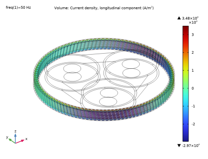
In the Settings window for 3D Plot Group, type Longitudinal Current Density (mf) in the Label text field.
3
Locate the Data section. From the Dataset list, choose Cut Plane 3.
4
Locate the Plot Settings section. From the View list, choose View 1 (Orthographic).
5
Locate the Color Legend section. Select the Show maximum and minimum values checkbox.
Volume 1
1
Right-click Longitudinal Current Density (mf) and choose Volume.
2
In the Settings window for Volume, locate the Data section.
3
From the Dataset list, choose Study 1/Solution 1 (sol1).
4
Click Replace Expression in the upper-right corner of the Expression section. From the menu, choose Component 1 (comp1) > Magnetic Fields > Currents and charge > Current density - A/m² > mf.Jz - Current density, z-component, (or just type “mf.Jz” in the Expression field).
Here, you have used the Replace Expression menu to find useful postprocessing variables. For many quantities predefined variables are available, and there is some auto-complete functionality too (try pressing Ctrl+Space, when typing variables in the Expression input field).
Selection 1
1
Right-click Volume 1 and choose Selection.
2
In the Settings window for Selection, locate the Selection section.
3
From the Selection list, choose Cable Armor.
4
In the Longitudinal Current Density (mf) toolbar, click  Plot.
Although View 5 (Perspective) tends to look more “impressive” due to the perspective distortion, we use the orthographic view View 1 (Orthographic) here, because it gives a clear overview of the situation. In a sense, this is a more pragmatic plot whereas the first one is more suitable for marketing purposes. To finish the plot, you can add some arrows to illustrate the field’s orientation.
Arrow Surface 1
1
In the Model Builder window, right-click Longitudinal Current Density (mf) and choose Arrow Surface.
2
In the Settings window for Arrow Surface, locate the Data section.
3
From the Dataset list, choose Study 1/Solution 1 (sol1).
4
Locate the Expression section. In the x-component text field, type 0.
5
In the y-component text field, type 0.
6
In the z-component text field, type mf.Jz.
7
From the Components to plot list, choose Tangential.
8
Click to expand the Title section. From the Title type list, choose None.
9
Locate the Arrow Positioning section. From the Placement list, choose Mesh vertices.
10
Locate the Coloring and Style section. From the Arrow type list, choose Cone.
11
From the Color list, choose Black.
Selection 1
1
Right-click Arrow Surface 1 and choose Selection.
2
In the Settings window for Selection, locate the Selection section.
3
From the Selection list, choose Armor, Exterior Boundaries.
4
In the Longitudinal Current Density (mf) toolbar, click  Plot.
5
Click the Zoom In button in the Graphics toolbar, twice.
The z-component of the current density has both positive and negative values, but may not show the kind of symmetry that you expected. You can investigate this further, by plotting expressions like real(mf.Jz), imag(mf.Jz) and abs(mf.Jz) — not included in the following instructions, but left as an exercise to the reader.
Since this is a frequency domain solution, the current density is a complex vector field where each vector component is actually a phasor rotating in the complex plane. In a plot like this you cannot actually see the complex values directly, but you can plot their norm or some kind of projection (like real() and imag() are doing). Just plotting “mf.Jz” will effectively do the same thing as real(mf.Jz).
Another trick you can use to get better insight in the full harmonic behavior of the solution is to make an animation. This is demonstrated in the Capacitive Effects and Inductive Effects tutorials, and in section Modeling Instructions — 3D Twist Model. For animations this plot is a bit on the heavy side though (rendering would take some time). Instead, let us add another plot for the transverse currents.
Transverse Current Density (mf)
1
In the Model Builder window, right-click Longitudinal Current Density (mf) and choose Duplicate.
2
In the Settings window for 3D Plot Group, type Transverse Current Density (mf) in the Label text field.
Volume 1
1
In the Model Builder window, expand the Transverse Current Density (mf) node, then click Volume 1.
2
In the Settings window for Volume, locate the Expression section.
3
In the Expression text field, type sqrt(real(mf.Jx)^2+real(mf.Jy)^2).
4
Select the Description checkbox. In the associated text field, type Transverse current density norm (instantaneous).
The expression used here is the instantaneous norm. It is an Euclidean norm, but not a complex norm. Therefore, it is still phase dependent. This norm is different from the variable mf.normB that you have used in the first plot. That one is a complex norm, defined as:  ||B|| =√ (B·B*)=(|Bx|2 + |By|2 + |Bz|2)1/2.
Arrow Surface 1
1
In the Model Builder window, click Arrow Surface 1.
2
In the Settings window for Arrow Surface, locate the Expression section.
3
In the x-component text field, type mf.Jx.
4
In the y-component text field, type mf.Jy.
5
In the z-component text field, type 0.
6
In the Transverse Current Density (mf) toolbar, click  Plot.
7
Click the Zoom Out button in the Graphics toolbar, twice.
Not that the kind of norm matters much in this case, it is still numerical noise you are looking at. The maximum value is on the order of 100–200 A/m2, which is about 2000 times less than what you would get from plotting the longitudinal component abs(mf.Jz).
This is important knowledge. It tells you that — when it comes to current densities in the armor at least — the margin of error of this model (and probably, models derived from it) is on the order of 100–200 A/m2.
Before you continue with the 3D twist model, it is good to perform a further validation. To this end, proceed with some volume integrals of the phase-, screen- and armor losses.
Phase Losses
1
In the Results toolbar, click  More Derived Values and choose Integration > Volume Integration.
2
In the Settings window for Volume Integration, type Phase Losses in the Label text field.
3
Locate the Selection section. From the Selection list, choose Phases.
4
Locate the Expressions section. In the table, enter the following settings:
5
Click  Evaluate.
Screen Losses
1
In the Results toolbar, click  More Derived Values and choose Integration > Volume Integration.
2
In the Settings window for Volume Integration, type Screen Losses in the Label text field.
3
Locate the Selection section. From the Selection list, choose Screens.
4
Locate the Expressions section. In the table, enter the following settings:
5
Click  Evaluate.
Armor Losses
1
In the Results toolbar, click  More Derived Values and choose Integration > Volume Integration.
2
In the Settings window for Volume Integration, type Armor Losses in the Label text field.
3
Locate the Selection section. From the Selection list, choose Cable Armor.
4
Locate the Expressions section. In the table, enter the following settings:
5
Click  Evaluate.
Table 3
1
Go to the Table 3 window.
The losses per kilometer should be about 47 kW, 12.6 kW, and 7.4 kW for the phases, screens, and armor respectively. Not precisely the same as the plain 2D model, but close. The overall accuracy seems to be about 0.5–1%, which is actually quite impressive for a 3D model with linear elements and a much coarser mesh.
Note that these are the total losses. You can evaluate mf.Qrh/Lsec and mf.Qml/Lsec too (the resistive-dielectric, and magnetic losses). For the armor, you will find the magnetic loss is about 10% of the total loss (for more on these loss terms, see the Thermal Effects tutorial). Furthermore, let us have a look at the lumped parameters.
Results
Phase AC Resistance
1
In the Results toolbar, click  Global Evaluation.
2
In the Settings window for Global Evaluation, type Phase AC Resistance in the Label text field.
3
Locate the Expressions section. In the table, enter the following settings:
4
Click  Evaluate.
Phase Inductance
1
In the Results toolbar, click  Global Evaluation.
2
In the Settings window for Global Evaluation, type Phase Inductance in the Label text field.
3
Locate the Expressions section. In the table, enter the following settings:
4
Click  Evaluate.
Table 5
1
Go to the Table 5 window.
The phase AC resistance per kilometer for the extruded 2D model should be about 52 mΩ, and the inductance should be about 0.41 mH. Again, quite impressive when compared to the plain 2D configuration presented in the Inductive Effects tutorial. Whether this kind of agreement may be expected can be investigated further if you like, by running the 2D models with linear elements and various mesh sizes.
Apart from the observation that this model seems legitimate (as legitimate as the 2D ones at least), the most important knowledge you gain here is that 0.5–1% is apparently a realistic margin of error. In the next section you will move into a domain where the 2D models cannot follow. By first modeling a case that the 2D models can reproduce, you have successfully validated your 3D model and obtained a fair estimate of its accuracy.
You have now finished the extruded 2D model. Save the resulting file, so that you can use it as a starting point for the next part.
From the File menu, choose Save.
Modeling Instructions — 3D Twist Model
Now things will get more interesting. The extruded 2D model from the previous section is modified to create a full 3D twist model. If you have just finished the previous section, you can continue where you left off. If you intend to start here, you will have to open a reference file from the Application Library. In both cases, it is convenient to resave the file under a new name (to avoid losing the extruded 2D model).
Root
1
From the File menu, choose Open.
2
3
From the File menu, choose Save As.
4
Browse to a suitable folder and type the filename submarine_cable_08_b_inductive_effects_3d.mph.
Results
Before adding the twist, it is good to have another look at the magnetic flux density. For the extruded 2D model the magnetic flux should be contained entirely in the cross section (the x,y-plane). In other words, the longitudinal component of the flux should be numerical noise (similar to the transverse current densities discussed previously). Let us validate that this is indeed the case.
Magnetic Flux Density, z-Component Norm (mf)
1
In the Model Builder window, under Results click Magnetic Flux Density Norm (mf).
2
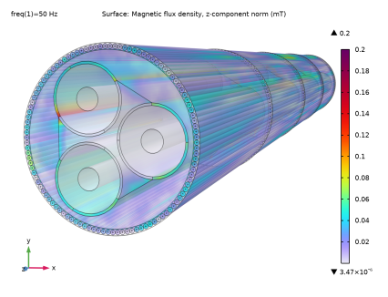
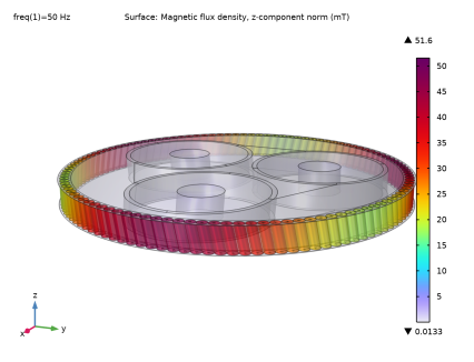
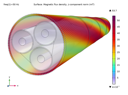
In the Settings window for 3D Plot Group, type Magnetic Flux Density, z-Component Norm (mf) in the Label text field.
Surface 1
1
In the Model Builder window, expand the Magnetic Flux Density, z-Component Norm (mf) node, then click Surface 1.
2
In the Settings window for Surface, locate the Expression section.
3
In the Expression text field, type abs(mf.Bz).
4
From the Unit list, choose mT.
5
Select the Description checkbox. In the associated text field, type Magnetic flux density, z-component norm.
Volume 1
1
In the Model Builder window, click Volume 1.
2
In the Settings window for Volume, locate the Expression section.
3
In the Expression text field, type abs(mf.Bz).
4
From the Unit list, choose mT.
5
In the Magnetic Flux Density, z-Component Norm (mf) toolbar, click  Plot.
The colors in the plot have no physical meaning whatsoever, but they do tell you something about the numerical properties of your model. Basically, this plot shows you how well the 3D model is capable of approximating a field that you know should be zero. The maximum value is on the order of 0.1–0.2 mT, which is about 250–300 times less than what you would get from plotting the magnetic flux density norm mf.normB.
It is fair to assume that this kind of accuracy will hold, even when the longitudinal component becomes nonzero later on. Notice that this is the third time we do a verification like this — the other two being based on the transverse current density, and a comparison with the highly detailed 2D model from the Inductive Effects tutorial. The previously established 0.5–1% still seems like a realistic margin of error. Next, proceed by enabling the twist.
Global Definitions
Please be aware that the geometry has been set to “Automatic rebuild”. Setting Nper to a large value and subsequently browsing in the Model Builder tree may freeze the COMSOL Desktop temporarily.
Geometric Parameters 3
1
In the Model Builder window, under Global Definitions click Geometric Parameters 3.
2
In the Settings window for Parameters, locate the Parameters section.
3
With the parameter Nper set to “1”, the following logic will come into motion:
The value of Nper will become an integer, causing the parameter Tenab (defined as round(Nper)==Nper) to become “1” (true).
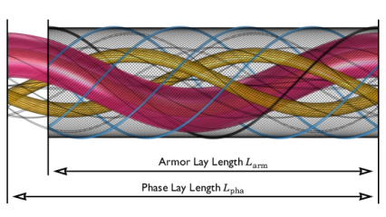
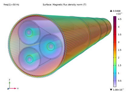
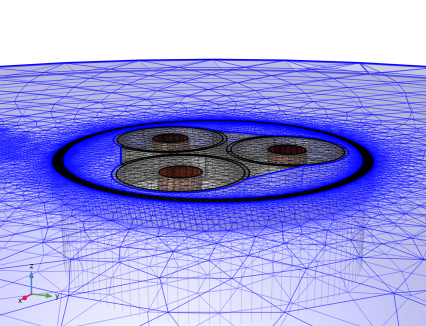
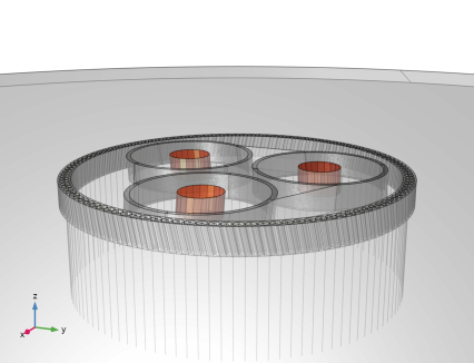
The length of the cable section included in the model Lsec (defined as CPcab*Nper) will increase tenfold. This sets the length of the geometry to be precisely one times the cable’s cross pitch (for more on this, see section On Lay Length and Cross Pitch).
The new parameter value Tenab will force the twist angle of the cable section Tsec (defined as 360[deg]*Tenab*Lsec/LLpha) to become “Lsec/LLpha” times one full revolution — note by the way that the expression 360[deg]*Tenab*Lsec/LLarm would have given you effectively the same angle.
In addition to this, Tenab will enable the slant correction factors SCFpha, and SCFarm, and will cause the two sweep operations in the geometry to generate helices instead of straight extrusions (as discussed in detail, in the Geometry & Mesh 3D tutorial).
Hint: If you press Ctrl+F and search for the strings “Nper”, “Tenab”, or “Lsec” in the model, you can see where these parameters have an effect.
The time required to build the geometry and the mesh will increase significantly, and the amount of degrees of freedom will increase about tenfold (settling around 3 MDOF). Solving the model should take about half an hour on a modern desktop machine. Let us proceed by rebuilding the geometry.
Geometry 1
1
In the Model Builder window, expand the Component 1 (comp1) node, then click Geometry 1.
2
In the Graphics window, check the geometry before rebuilding it.
The cable looks shorter as it did before, because the camera is using the latest parameter values while the geometry has not yet been rebuilt. In fact, View 5 (Perspective) is now showing the cable as it actually is, while the first four views show a compacted version. The initial rebuild should take about 5 minutes or so, but subsequent rebuilds should be quicker due to caching.
3
In the Geometry toolbar, click  Build All.
The cable geometry is now about 1.6 m long, with an opposite twist for the phases and the armor. This will be the geometry used for this tutorial section, and the two that follow (Linearized Resistivity, and Compensated Stabilization).
Mesh 1
1
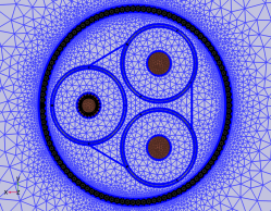
In the Model Builder window, under Component 1 (comp1) right-click Mesh 1 and choose Build All (this should take a couple of minutes).
2
Right-click Component 1 (comp1) > Mesh 1 and choose Statistics.
3
In the Settings window for Mesh, check the following statistics:
The actual numbers you get will probably deviate (by less than a percent), and will depend on your operating system, COMSOL version, and geometry representation — COMSOL kernel, or CAD kernel.
As far as meshes go, this one does not give the best statistics. Not when considering the Element Quality Histogram at least. Ideally, it should be a nice bell shape with a not-too-large standard deviation and a good average element quality. Here, “good” means the aspect ratio of the elements should be close to 1. Assuming your material properties and your physics are fairly isotropic, an isotropic mesh will lead to a friendly matrix structure; iterative solvers should like it.
This reasoning is very general however — as COMSOL is able to handle a vast amount of different kinds of physics — and the element quality measure does not take into account the extreme aspect ratio of the features included in the cable. If you would put a nice isotropic tetrahedral mesh in this model (while still resolving the skin depth of course), the amount of degrees of freedom would quickly rise to 30 million or more. Although iterative solvers may still be able to handle that, it turns out not to be the most efficient way to go about.
Instead, this mesh has been optimized to a great extent, to be used with a direct solver — more precisely: PARDISO (MUMPS should work too, if pivoting is limited). Direct solvers are more forgiving when it comes to the mesh quality, but they do consume more memory. Luckily, desktop machines with 32–64 GB of RAM and several hundred gigabytes of SSD swap drive capacity are very affordable nowadays (2019).
So the main goal has been to find a mesh that resolves the geometry and the physics as best as possible, while still keeping the DOF count low enough to have a reasonable solving time on a modern desktop machine. This is actually one of the more challenging exercises in this tutorial series, see the Geometry & Mesh 3D tutorial.
Let us continue with some coordinate systems and variable definitions.
Definitions
Rotated System 2 (sys2)
1
In the Definitions toolbar, click  Coordinate Systems and choose Rotated System.
2
In the Settings window for Rotated System, locate the Rotation section.
3
Find the Euler angles subsection. In the α text field, type Tsec.
This rotated coordinate system will be used in the Periodic Condition, to apply a twist with an angle equal to Tsec. That is; the model is periodic, but with a twist. This is due to the dissimilar lay length of the phases, and the armor (see section On Lay Length and Cross Pitch). Full periodicity would require models as long as 35 m, with over 30 MDOF. The science behind this has been discussed in detail in reference [2].
Cylindrical System 3 (sys3)
1
In the Definitions toolbar, click  Coordinate Systems and choose Cylindrical System.
(This coordinate system is used to simplify the variable expressions that will follow).
Armor Wire Variables
1
In the Model Builder window, right-click Definitions and choose Variables.
2
In the Settings window for Variables, type Armor Wire Variables in the Label text field.
3
Locate the Geometric Entity Selection section. From the Geometric entity level list, choose Domain.
4
From the Selection list, choose Cable Armor.
5
Locate the Variables section. Click  Load from File.
6
These variables will be very useful during postprocessing, when investigating the different kinds of magnetic flux and current flowing through the armor. The vector field e_awx,y,z is basically the φ unit vector — as taken from the cylindrical coordinate system sys3 — that is subsequently scaled and given a z-component, such that it follows the helical paths of the armor wires.
Consequently, the inner product BL = eaw·B will give the value of the longitudinal magnetic flux density component, and BL = eawBL will give the entire longitudinal magnetic flux density vector field. The transverse magnetic flux density is then defined as BT = B BL. The same procedure is repeated for the currents. Finally, some instantaneous and absolute (complex) norms are added for easy plotting.
Proceed by updating the periodic condition. Enable the advanced physics options to get access to the Orientation of Source and Orientation of Destination sections.
Root
1
Click the  Show More Options button in the Model Builder toolbar.
2
In the Show More Options dialog, in the tree, select the checkbox for the node Physics > Advanced Physics Options.
3
Magnetic Fields (mf)
Periodic Condition 1
1
In the Model Builder window, expand the Component 1 (comp1) > Magnetic Fields (mf) node, then click Periodic Condition 1.
2
In the Settings window for Periodic Condition, click to expand the Orientation of Source section.
3
From the Transform to intermediate map list, choose Global coordinate system.
4
Right-click Component 1 (comp1) > Magnetic Fields (mf) > Periodic Condition 1 and choose Manual Destination Selection.
5
Locate the Destination Selection section. From the Selection list, choose Cross Section, Top.
6
In the Graphics window toolbar, clicknext to  Go to Default View, then choose Go to View 1 (Orthographic).
7
Click the  Zoom to Selection button in the Graphics toolbar.
8
Click to expand the Orientation of Destination section. From the Transform to intermediate map list, choose Rotated System 2 (sys2).
Input 1
1
In the Model Builder window, expand the Component 1 (comp1) > Magnetic Fields (mf) > Phase 1 > Geometry Analysis 1 node, then click Input 1.
2
In the Settings window for Input, locate the Input section.
3
Select the Slanted cut checkbox.
Output 1
1
In the Model Builder window, click Output 1.
2
In the Settings window for Output, locate the Output section.
3
Select the Slanted cut checkbox.
Phase 2, Phase 3
1
Repeat these steps for Phase 2, and Phase 3.
Now that the phase conductors have a twist, the currents do not flow normal to the periodicity plane any more. The Slanted cut setting is there to relax the input and output constraints accordingly.
With the updated geometry and mesh, some new coordinate systems and postprocessing variables, and a twisted periodic condition, you are all set and ready for some proper numerical analysis. Before going ahead with solving however, there is one thing you might want to have a look at; more statistics.
Study 1
Solution 1 (sol1)
1
In the Model Builder window, expand the Study 1 > Solver Configurations > Solution 1 (sol1) node.
2
Right-click Study 1 > Solver Configurations > Solution 1 (sol1) > Compile Equations: Frequency Domain and choose Statistics.
3
In the Settings window for Compile Equations, check the following statistics:
As with the mesh statistics, your values will probably deviate a little.
The Magnetic vector potential (comp1.A) variable is clearly the main degree of freedom. Its DOF count is related to the discretization order chosen in the Settings window for the Magnetic Fields interface (see section Shape Functions and Discretization Order). Furthermore, the DOF count depends on the kind of shape function — curl elements in this case, Lagrange elements for the 2D models — and the number and type of mesh elements (tetrahedra, pyramids, prisms, and so on). For more on this, see the AC/DC Module User’s Guide, or the COMSOL Multiphysics Reference Manual.
The DOF count has been decreased significantly, by choosing a linear discretization order and by optimizing the mesh. This is a very common strategy for larger finite element models, especially when direct solvers and nonlinear materials are involved. Nonlinear materials are not included here, but can easily be added using refs. [2, 4, 5].
According to a general rule of thumb, for a direct solver the memory requirements and overall computational effort should scale with the number of degrees of freedom, squared. It also depends on the sparsity of the matrix however, and whether it is ill-conditioned. Pushing the DOF count down too far, may harm both speed and accuracy. 3 MDOF is chosen as a “fair compromise” for this model, and any derivative you might want to base on it.
The other degrees of freedom are related to computing the external electric field Eext needed to excite the phase currents (for more on this, see the previous section Extruded 2D Model). Let us proceed by computing the solution.
In the Home toolbar, click Compute.
This procedure should take about half an hour, assuming a modern desktop machine with an SSD and 32 GB of RAM (or more).
First, the Coil Geometry Analysis study step will solve a diffusion problem to determine the electric field needed to excite the phases. This should only take a minute and consume about 4–6 GB of RAM.
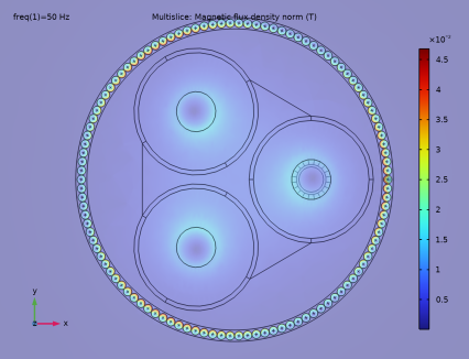
Then, the Frequency Domain study step will solve for the magnetic vector potential. The three coil ODE variables are included as well, allowing the system to tune the excitation such that the phase currents match the desired values: I0, I0*exp(-120[deg]*j), and I0*exp(+120[deg]*j).
During this process, the direct solver is likely to go out-of-core. This means, (part of) the LU factorization is written to your disk — to the folder for temporary files, as set in the COMSOL Preferences window.
The memory consumption may go up to about 80–90% of your system capacity, but no more than 100–120 GB. When written on disk, the LU factorization should take about 90–100 GB.
Results
Magnetic Flux Density, z-Component Norm (mf)
1
In the Model Builder window, under Results click Magnetic Flux Density, z-Component Norm (mf).
2
In the Magnetic Flux Density, z-Component Norm (mf) toolbar, click  Plot.
As you can see, the longitudinal component of the flux is far from numerical noise now. In fact, the flux is predominantly in the z direction (in the armor, that is). You can investigate this further by plotting and comparing expressions like mf.normB, normBL, and normBT.
The results can be understood as follows: The magnetic field H encircles the phase conductors. This is true by definition — as dictated by Ampère’s law ×H = J — and can clearly be seen in the 2D models. At the same time, the magnetic flux density B will try to find the path of least reluctance. Due to this, the flux lines will quickly find their way to the magnetic armor and then travel along the armor wires for a while, to make their way around the phase conductor (as discussed in refs. [2, 6]).
For the 2D models the only available option for the flux lines, is to hop from one armor wire to another. Now, with the opposing twist, traveling a short distance along the armor wire has become a viable alternative. Although most of the flux seems to be going for this option now, the armor wire variable normBT will show you that hopping is still an option too.
It is therefore useful to distinguish two different kinds of flux, the longitudinal flux BL and the transverse flux BT (see Figure 6). The longitudinal flux is linked to the transverse current density JT in the armor wires (small circular eddies), and the transverse flux is linked to longitudinal currents JL. In the 2D and 2.5D models, you will only see the transverse flux and the longitudinal currents.
The ratio between the two, is dictated by the ratio of the reluctance of the two paths. Increasing the gap between the wires will benefit the longitudinal flux, and increasing the cable’s cross pitch (or decreasing the armor’s permeability) will benefit the transverse flux. This may also present a challenge for the model’s accuracy: If the armor wires are touching (if there is a negligible film of bitumen in-between), it may be difficult to get an accurate value for the gap size and the gap’s effective permeability. This is true for contact problems in general, not just magnetic ones.
You can verify quite easily exactly how sensitive this model is to the magnetic properties of the gap, by creating a duplicate of the Generic insulator material, adding it to the domain in-between the wires, and varying its permeability. If you know very little about the gap’s properties but you do know the inductance of the cable, one useful trick is to tune the permeability between the wires until the cable’s inductive properties match the required value.
Generally speaking, having a good magnetic connection between the wires should be avoided regardless. The armor would start behaving like a magnetic core, and the inductance and losses would increase significantly. Some cable designs include polyethylene (PE) spacer rods, replacing part of the armor wires [6]. For those designs, the contact problem does not occur.
Please proceed by investigating the armor currents.
Volume 1
1
In the Model Builder window, expand the Results > Longitudinal Current Density (mf) node, then click Volume 1.
2
In the Settings window for Volume, locate the Expression section.
3
In the Expression text field, type JL.
Arrow Surface 1
1
In the Model Builder window, click Arrow Surface 1.
2
In the Settings window for Arrow Surface, locate the Expression section.
3
In the x-component text field, type JLx.
4
In the y-component text field, type JLy.
5
In the z-component text field, type JLz.
6
In the Longitudinal Current Density (mf) toolbar, click  Plot.
7
Click the Zoom In button in the Graphics toolbar, twice.
The plot is phase dependent and shows both positive and negative currents. Since the armor wires are twisted around the phase conductors, each wire will be subjected to the electromotive force (emf) of all phases, to the same degree. Assuming the cable is well-balanced, and assuming the electrical contact between the wires is negligible, the total longitudinal current per armor wire will be approximately zero. This reasoning is the basis for the 2.5D models — see the Inductive Effects tutorial, and reference [7].
As the total current per wire is about zero, the current must flow back and forth within the wire’s cross section. On the inside of the armor ring where the emf of the local phase conductor is strongest, the currents will flow in the direction dictated by the emf. On the outside, the currents will flow back. This causes the plot to show different shades of purple: As soon as the plot turns red on one side of the wire, it will turn blue on the other side.
Volume 1
1
In the Model Builder window, expand the Results > Transverse Current Density (mf) node, then click Volume 1.
2
In the Settings window for Volume, locate the Expression section.
3
In the Expression text field, type normJTi.
Arrow Surface 1
1
In the Model Builder window, click Arrow Surface 1.
2
In the Settings window for Arrow Surface, locate the Expression section.
3
In the x-component text field, type JTx.
4
In the y-component text field, type JTy.
5
In the z-component text field, type JTz.
6
In the Transverse Current Density (mf) toolbar, click  Plot.
This plot is phase dependent too, but only shows positive values. That is because the definition for the instantaneous transverse current density norm as given in Armor Wire Variables, is incapable of making a distinction between a clockwise (positive) and counterclockwise (negative) direction. Naturally, the eddies will oscillate between clockwise and counterclockwise, as the longitudinal flux density in the armor oscillates between positive and negative values.
You can investigate the direction of the eddies further by looking at the arrows. They should correspond to jωBL, or dBL/dt in the armor. In other words, if you combine a volume plot of -mf.iomega*BL with an arrow plot of JTx,y,z, you will see they correlate — not included in the following instructions, but left as an exercise to the reader.
In fact, you can use this to your advantage and obtain a signed expression for the instantaneous transverse current density: if(-mf.iomega*BL>0,1,-1)*normJTi. Here, normJTi will give a magnitude as a function of phase, and the sign of -mf.iomega*BL will tell you whether it should be (counter) clockwise.
Volume 1
1
In the Model Builder window, click Volume 1.
2
In the Settings window for Volume, locate the Expression section.
3
In the Expression text field, type if(-mf.iomega*BL>0,1,-1)*normJTi.
4
In the Description text field, type Current density, transverse component.
5
In the Transverse Current Density (mf) toolbar, click  Plot.
6
Click the Zoom Out button in the Graphics toolbar, twice.
In order to get a good understanding of the full dynamic behavior of the currents, you can make an animation. The animation will need to render a number of frames, and for that the 3D plots are a bit on the heavy side (besides, the 3D plots would give too much detail for a good movie). Instead, we add a lightweight 2D plot with a height expression showing both kinds of currents in one picture.
Surface 1
1
In the Results toolbar, click  More Datasets and choose Surface.
2
In the Settings window for Surface, locate the Parameterization section.
3
From the x- and y-axes list, choose xy-plane.
4
Locate the Selection section. From the Selection list, choose Cable Ring, Top.
5
In the Graphics window toolbar, clicknext to  Go to Default View, then choose Go to View 5 (Perspective).
The 2D plot will be based on a cross section of the armor ring.
Longitudinal and Transverse Current Density (mf)
1
In the Results toolbar, click  2D Plot Group.
2
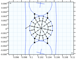
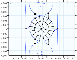
In the Settings window for 2D Plot Group, type Longitudinal and Transverse Current Density (mf) in the Label text field.
3
Locate the Data section. From the Dataset list, choose Surface 1.
4
Locate the Color Legend section. Select the Show maximum and minimum values checkbox.
The empty plot will show the contours of the dataset, the dataset edges. You can enable and disable them in the Settings window for 2D Plot Group. The goal here is to put two plots in one. You can mimic a second set of dataset edges, by adding a black line plot and equipping it with a deformation.
Line 1
1
Right-click Longitudinal and Transverse Current Density (mf) and choose Line.
2
In the Settings window for Line, locate the Expression section.
3
In the Expression text field, type 1.
4
Click to expand the Title section. From the Title type list, choose None.
5
Locate the Coloring and Style section. From the Coloring list, choose Uniform.
6
From the Color list, choose Black.
Deformation 1
1
Right-click Line 1 and choose Deformation.
2
In the Settings window for Deformation, locate the Expression section.
3
In the x-component text field, type x.
4
In the y-component text field, type y.
5
Locate the Scale section.
6
Select the Scale factor checkbox. In the associated text field, type 0.1.
7
In the Longitudinal and Transverse Current Density (mf) toolbar, click  Plot.
8
Click the  Zoom Extents button in the Graphics toolbar.
Now, you have two concentric circles. The x- and y-components of the deformation expression are parts of a displacement vector, so typing in numbers will just give you a constant displacement. If you type in functions of the coordinates x and y however, you can apply scaling. Applying a displacement of “x” at coordinate x, means moving to “2x”. So the second ring will be twice as big. Subsequently, the scaling is fine-tuned by setting the Scale factor to 0.1. The Deformation node is typically used by Structural Mechanics models, where the deformation is actually part of the solution.
Surface 1
1
In the Model Builder window, right-click Longitudinal and Transverse Current Density (mf) and choose Surface.
2
In the Settings window for Surface, locate the Expression section.
3
In the Expression text field, type JL.
4
Locate the Coloring and Style section. From the Color table list, choose Dipole.
5
From the Scale list, choose Linear symmetric.
Height Expression 1
1
Right-click Surface 1 and choose Height Expression.
2
In the Settings window for Height Expression, locate the Axis section.
3
Select the Scale factor checkbox. In the associated text field, type 5E-7.
4
In the Longitudinal and Transverse Current Density (mf) toolbar, click  Plot.
5
Click the  Show Grid button in the Graphics toolbar once (to hide the grid).
6
Click the  Go to Default View button in the Graphics toolbar.
The longitudinal current density moves back and forth within the cross section with an average hovering around zero, as discussed before.
Surface 2
1
In the Model Builder window, under Results > Longitudinal and Transverse Current Density (mf) right-click Surface 1 and choose Duplicate.
2
In the Settings window for Surface, locate the Expression section.
3
In the Expression text field, type if(-mf.iomega*BL>0,1,-1)*normJTi.
4
Select the Description checkbox. In the associated text field, type Current density, transverse component.
5
Click to expand the Inherit Style section. From the Plot list, choose Surface 1.
6
Clear the Deform scale factor checkbox.
Now, you can move the transverse current density plot to the outer ring, by giving it the same deformation as Line 1.
Deformation 1
In the Model Builder window, under Results > Longitudinal and Transverse Current Density (mf) > Line 1 right-click Deformation 1 and choose Copy.
Deformation 1
1
In the Model Builder window, right-click Surface 2 and choose Paste Deformation.
2
In the Longitudinal and Transverse Current Density (mf) toolbar, click  Plot.
3
Click the  Go to Default View button in the Graphics toolbar.
4
In the Model Builder window, click Deformation 1.
The whole thing is phase dependent, which means you can animate it by sweeping over the phase.
Animation 1
1
In the Results toolbar, click  Animation and choose Player.
2
In the Settings window for Animation, locate the Scene section.
3
From the Subject list, choose Longitudinal and Transverse Current Density (mf).
4
Locate the Animation Editing section. From the Sequence type list, choose Dynamic data extension.
5
Locate the Frames section. In the Number of frames text field, type 60.
6
Locate the Playing section. From the Repeat list, choose Forever.
7
Click the  Play button in the Graphics toolbar (see the animation from ref. [9]).
The transverse current density forms cones, with the circulating current increasing in magnitude as you get closer to the outer perimeter of the armor wire’s cross section. The cones are not exactly “straight”. Instead, the decay of the current density field as you get further into the wire, follows the logic of a strongly attenuated wave phenomenon (as expected for a skin effect).
The amplitude of the oscillation (both for JL and JT), depends on the location of the armor wire with respect to the phases. You can see the amplitude by replacing the expressions JL and if(-mf.iomega*BL>0,1,-1)*normJTi, by normJL and normJT (although this would mean losing phase dependency). Let us add a plot for the screen and armor losses as well.
8
Click the Stop button in the Graphics toolbar.
Volumetric Loss Density, Electromagnetic (mf)
1
In the Results toolbar, click  3D Plot Group.
2
In the Settings window for 3D Plot Group, type Volumetric Loss Density, Electromagnetic (mf) in the Label text field.
3
Locate the Data section. From the Dataset list, choose Cut Plane 3.
4
Locate the Plot Settings section. From the View list, choose View 5 (Perspective).
5
Locate the Color Legend section. Select the Show maximum and minimum values checkbox.
Volume 1
1
Right-click Volumetric Loss Density, Electromagnetic (mf) and choose Volume.
2
In the Settings window for Volume, locate the Data section.
3
From the Dataset list, choose Study 1/Solution 1 (sol1).
4
Locate the Expression section. In the Expression text field, type mf.Qh.
5
Locate the Coloring and Style section. From the Color table list, choose Disco.
Selection 1
1
Right-click Volume 1 and choose Selection.
2
In the Settings window for Selection, locate the Selection section.
3
From the Selection list, choose Screens.
4
In the Volumetric Loss Density, Electromagnetic (mf) toolbar, click  Plot.
The screen loss reaches a minimum at the center of the cable, where the electromotive force from the three phase conductors cancels out. This is very similar to what the 2D models would show you.
Volume 2
1
In the Model Builder window, under Results > Volumetric Loss Density, Electromagnetic (mf) right-click Volume 1 and choose Duplicate.
2
In the Settings window for Volume, click to expand the Title section.
3
From the Title type list, choose None.
4
Locate the Coloring and Style section. From the Color table list, choose HeatCamera.
Selection 1
1
In the Model Builder window, expand the Volume 2 node, then click Selection 1.
2
In the Settings window for Selection, locate the Selection section.
3
Click to select the  Activate Selection toggle button.
4
From the Selection list, choose Cable Armor.
5
In the Volumetric Loss Density, Electromagnetic (mf) toolbar, click  Plot.
The armor loss shows the same spatial distribution as the magnetic flux density and the currents: trails of loss concentration are spiraling around the cable’s axis. They follow the helical paths of the phase conductors, rather than those of the armor wires themselves.
No 2D (or 2.5D) model would be able to capture this effect, but that does not render them useless. Proceed by investigating how this model compares to the 2D and 2.5D models.
Phase Losses
1
In the Model Builder window, expand the Results > Derived Values node, then click Phase Losses.
2
In the Settings window for Volume Integration, locate the Expressions section.
3
In the table, update the description. Type Phase losses (3D twist model), that is; replace “extruded 2D” with “3D twist”.
4
In the Settings window for Volume Integration, click Evaluate.
Screen Losses, Armor Losses, Phase AC Resistance, and Phase Inductance
Repeat these steps for Screen Losses, Armor Losses, Phase AC Resistance, and Phase Inductance.
Table
1
Go to the Table window.
The losses per kilometer should be about 48 kW, 17.5 kW, and 2.8 kW for the phases, screens, and armor respectively. This is reflected by an increased AC resistance: 53 mΩ. The inductance increases too, to 0.44 mH. Note that if you evaluate the resistive- and magnetic losses in the armor separately (using mf.Qrh and mf.Qml), you will see the magnetic loss has tripled; it now represents over 70% of the total armor loss.
2
Let us compare these figures with those from the Inductive Effects tutorial (submarine_cable_04_inductive_effects.mph):
As you can see, the loss balance in the phases, screens and armor is “wrong” for the plain 2D configuration. The armor losses are greatly overestimated, and the screen losses are underestimated.
This does not keep the 2D model from giving a pretty accurate figure for the total loss though. And the same goes for the AC resistance. One may argue it gives the “right” value for the “wrong” reasons, and that might be an issue for academic applications. As an engineering solution however, the 2D model is still a perfectly legitimate tool, and only for a fraction of the computational effort: one minute, rather than half an hour.
Although the loss and resistance of the 2D model may serve as a good approximation, the inductive properties are way off. Luckily, the opposite is true for the 2.5D model with Milliken phase conductors (and the 2.5D model without Milliken): They do not provide a very good figure for the resistance, but the inductance is actually quite close. This kind of behavior is confirmed by reference [2], where 2D, 2.5D and 3D models have been compared to measurements.
In practice, 3D models would typically be used by cable manufacturers and academics who feel the need to get a good understanding of the physics involved (or to validate their 2D models). 2D and 2.5D models might be more suitable for end users of cable systems who intend to investigate whether their cable duct provides adequate cooling, for example.
The good correspondence between the 2D models and the 3D one will be very useful for the next part of this tutorial by the way. In the next section, we will take the temperature readings from the fully coupled induction heating model discussed in the Thermal Effects tutorial, and use them in a 3D model to apply a temperature correction. This temperature correction will effectively heat up the cable to nominal operating conditions.
You have now finished the 3D twist model. Save the resulting file, so that you can use it as a starting point for the next part.
From the File menu, choose Save.
Modeling Instructions — Linearized Resistivity 3D
With the 3D twist model up and running, the biggest hurdle has been taken. It is not yet an accurate representation of a cable system under nominal operating conditions however, as it currently operates at room temperature (20°C, or 293.15 K). Nominal conditions assume 80–90°C. A common procedure is to take measured or modeled temperature readings (or temperature values from literature), and apply a first-order temperature correction to the conductivity. This is typically done using linearized resistivity.
The following will show you how to implement this. If you have just finished the previous section, you can continue where you left off. If you intend to start here, you will have to open a reference file from the Application Library. In both cases, it is convenient to resave the file under a new name (to avoid losing the 3D twist model).
Root
1
From the File menu, choose Open.
2
3
From the File menu, choose Save As.
4
Browse to a suitable folder and type the filename submarine_cable_08_c_inductive_effects_3d.mph.
Global Definitions
The expected temperatures have been stored in a file, together with the parameters used for the temperature dependent conductivity.
Thermal Parameters
1
In the Home toolbar, click  Parameters and choose Add > Parameters.
2
In the Settings window for Parameters, type Thermal Parameters in the Label text field.
3
Locate the Parameters section. Click  Load from File.
4
Twelve new parameters have been added, with the last seven being the ones used for temperature dependent material properties. The parameters Tmcon, Tmpbs, and Tmarm are the expected average temperatures for the phases, screens and armor, respectively. They have been obtained from the fully coupled induction heating model discussed in the Thermal Effects tutorial.
That model is a plain 2D model, not a 3D one. But since the plain 2D models have given pretty accurate values for the total loss at room temperature, they are expected to do so at elevated temperatures as well. Because the raise in temperature is strongly tied to the generated loss, the 2D models should give pretty accurate values for the phase, screen and armor temperatures — indeed, note that these numbers agree fairly well with those used in reference [4].
Proceed by enabling the Advanced Physics Options, to get access to the Model Input section.
Root
1
Click the  Show More Options button in the Model Builder toolbar.
2
In the Show More Options dialog, in the tree, select the checkbox for the node Physics > Advanced Physics Options.
3
Magnetic Fields (mf)
Phase 1
The settings window for the coil feature contains a lot of sections. For many of these, the default settings are sufficient. Collapse them to have a closer look at the important part; the Constitutive Relation Jc-E section.
1
In the Model Builder window, expand the Component 1 (comp1) > Magnetic Fields (mf) node, then click Phase 1.
2
Click to collapse the Material Type section, the Coordinate System Selection section, the Constitutive Relation B-H section, and the Constitutive Relation D-E section.
Next, proceed by setting the conduction model and the temperature.
3
In the Settings window for Domain Coil, locate the Constitutive Relation Jc-E section.
4
From the Conduction model list, choose Linearized resistivity.
5
Click to expand the Model Input section. From the T list, choose User defined. In the associated text field, type Tmcon.
In this case, linearized resistivity is combined with a preset temperature. This requires you to decouple the used temperature from the Common model input and define your own.
You can consider the common model inputs to be a central database of physical conditions. When a model contains a Heat Transfer interface for example, that interface will announce the output temperature to the model inputs. Another part of the model — like a temperature dependent material property — is then able to retrieve the temperature as a model input.
Phase 2, Phase 3
Repeat these steps for Phase 2, and Phase 3.
Next, will be the screens and the armor. For this, you will have to introduce more Ampère’s Law features. The reasoning behind this, is as follows: The default Ampère’s Law feature (with default settings) is applied to all domains within the selection of the physics interface. You cannot clear its selection. This ensures there are equations to solve for (the problem would be singular otherwise). Something similar holds for Magnetic Insulation being the default exterior boundary condition.
Now, if you intend to have the same behavior for all passive domains (as was the case for the models discussed in the previous sections), you can just modify the default features. But if you intend to have “special” settings for certain domains only — like a remanent flux density Br, a nonlinear magnetic curve, or in this case, linearized resistivity — you will have to override the default behavior by adding more physics features.
In some cases, overriding is not necessary though. A contribution to the default behavior may be enough. The External Current Density is an example of such a case. It adds an additional contribution Je to the set of equations already introduced by the Ampère’s Law feature. To see how features override or contribute, you can check the Override and Contribution section in the Settings window.
Screens
1
In the Physics toolbar, click  Domains and choose Ampère’s Law in Solids.
2
In the Settings window for Ampère’s Law in Solids, type Screens in the Label text field.
3
Locate the Domain Selection section. From the Selection list, choose Screens.
The settings window for the Ampère’s Law feature contains a lot of sections. For many of these, the default settings are sufficient. Collapse them to have a closer look at the important part; the Constitutive Relation Jc-E section.
4
Click to collapse the Coordinate System Selection section, the Constitutive Relation B-H section, and the Constitutive Relation D-E section.
Next, proceed by setting the conduction model and the temperature.
5
Locate the Constitutive Relation Jc-E section. From the Conduction model list, choose Linearized resistivity.
6
Click to expand the Model Input section. From the T list, choose User defined. In the associated text field, type Tmpbs.
Cable Armor
1
Right-click Screens and choose Duplicate.
2
In the Settings window for Ampère’s Law in Solids, type Cable Armor in the Label text field.
3
Locate the Domain Selection section. From the Selection list, choose Cable Armor.
4
Locate the Model Input section. In the T text field, type Tmarm.
Materials
Now, you will see that COMSOL starts detecting missing material properties. The properties that should be added are listed in the following table. Please check all of them for the correct value, even the ones that are already filled in. Note that for cases like this, a convenient option is to copy-paste the values directly from this *.pdf file to COMSOL.
1
In the Model Builder window, under Component 1 (comp1) > Materials, add the following material properties:
The reference resistivity for copper is divided by Ncon. This is because the phase conductors consist of compacted strands, rather than solid copper. For more information on this, see the Inductive Effects tutorial.
Now, let us investigate the results.
Study 1
In the Study toolbar, click  Compute.
Results
Magnetic Flux Density, z-Component Norm (mf)
When compared to the results from the 3D twist model at room temperature, there is a small raise of the magnetic flux density in the armor (we will get back to this). Otherwise, the Magnetic Flux Density, z Component Norm (mf) plot looks pretty much unchanged.
In order to make a good comparison, proceed by reevaluating the losses, the AC resistance, and the inductance.
Phase Losses
1
In the Model Builder window, expand the Results > Derived Values node, then click Phase Losses.
2
In the Settings window for Volume Integration, locate the Expressions section.
3
In the table, update the description. Type Phase losses (linres 3D), that is; replace “3D twist model” with “linres 3D”.
4
In the Settings window for Volume Integration, click Evaluate.
Screen Losses, Armor Losses, Phase AC Resistance, and Phase Inductance
Repeat these steps for Screen Losses, Armor Losses, Phase AC Resistance, and Phase Inductance.
Table
1
Go to the Table window.
The losses per kilometer should be about 59 kW, 14.7 kW, and 2.8 kW for the phases, screens, and armor. The magnetic loss in the armor has increased again; it now represents over 75% of the total armor loss. Due to the elevated temperatures, the overall loss in the cable’s cross section has increased by about 12%. This is reflected by an increased AC resistance: 59 mΩ. The inductance increases slightly, to 0.45 mH.
2
Now, let us make a comparison with the results from the 3D twist model discussed previously, and the fully coupled induction heating model discussed in the Thermal Effects tutorial (submarine_cable_06_thermal_effects.mph):
Linearized Resistivity 3D vs. 3D Twist Model
So compared to the 3D twist model at room temperature, the phase losses went up by 23%. This is according to expectations. A crude guess based on the expression for linearized resistivity Equation 12 would give you 1+ALcup*(Tmcon-Tmref), which evaluates to a 27% increase. If you would assume Q = I2Rdc to be valid, a 27% increase in resistivity would mean a 27% increase in loss.
This kind of reasoning is only valid under stationary conditions however (as discussed in the Thermal Effects tutorial). For nonzero frequencies, different rules apply. In the frequency domain there will always be both an applied and an induced current. For the applied currents in the current-driven phase conductors the Q = I2R reasoning will still hold (or Q = |I|2R/2 rather), but not for the induced currents.
This is because induced currents are voltage driven (driven by the electromotive force from the applied currents), and they will follow Q = |V|2/(2R) instead. For induced currents, a higher resistance means less current, means reduced loss. Since the phase conductors carry both applied and induced currents — and since the loss is given by the sum of both — the increase is large, but not as large as 27%.
As opposed to the phases, the screens only carry induced currents (they are passive conductors) so one would expect the losses to go down. They do, but not as much as you would expect based on 1+ALpbs*(Tmpbs-Tmref). This is because the reduced induced phase currents are now less effective in screening the fields coming from the applied phase currents. So the lead sheath will perceive a stronger emf coming from the phases.
For the armor, there is yet another complication. The armor is a passive conductor too, so here too you would expect the losses to go down, but they do not. Instead, they stay more or less the same. The armor develops a larger electric resistivity indeed, causing the resistive losses to go down. At the same time, however, the magnetic losses increase further. These losses are caused by a stronger magnetic flux density in the armor, as seen earlier in the Magnetic Flux Density, z Component Norm (mf) plot.
Linearized Resistivity 3D vs. Coupled Induction Heating
Comparing the 2D and 3D models at elevated temperatures, results in more or less the same conclusions as comparing them at room temperature, see Modeling Instructions — 3D Twist Model. That is; in 2D the screen losses are underestimated, the armor losses are overestimated but the total loss and AC resistance are remarkably similar.
Perhaps a more interesting question would be, whether this solution is self-consistent: What would happen if you would take the 3D phase, screen and armor loss which is clearly not the same for 2D and 3D and dump it into a 2D Heat Transfer model? Would that give the same temperatures as the ones you put into the 3D model? It turns out, the answer is “no”, but it is close.
This model applies a first-order temperature correction, but you can also go for a second-order temperature correction. If you put the losses from this 3D model in a fully detailed 2D thermal model, the phase and screen temperatures will go up by about 1°C, and the average armor temperature will stay more or less the same. If you then put those temperatures back into your 3D model, your total loss will go up by 100–200 W/km, or about 0.2%. In the previous two sections of this tutorial we have already established that the overall accuracy of this 3D model is likely to be on the order of 0.5–1%, so on second thought doing a second-order temperature correction may not be that interesting.
It does show however, that a 3D electromagnetic model and a 2D thermal model can be made self-consistent — you could build a hybrid 2D/3D fully coupled induction heating model. This is a very interesting approach as 2D seems more suitable for the thermal part of the device. More suitable because the thermal problem is dominated by the insulators, rather than the conductors (much like the electrostatics problem discussed in the Capacitive Effects tutorial).
Speaking about accuracy, there is still one loose end that is worth having a look at. In the section Modeling Instructions (including Modeling Instructions Extruded 2D Model), you have set the conductivity of the “generic insulator” material to 50[S/m]. Why this is necessary and how it affects accuracy, is discussed in the next section.
You have now finished the 3D twist model with first-order temperature correction. Save the resulting file, so that you can use it as a starting point for the next part.
From the File menu, choose Save.
Modeling Instructions — Compensated Stabilization
The finite insulator conductivity is necessary, because the numerical system would not be able to determine a unique solution for the magnetic vector potential A otherwise (not with the used solver at least). When the Helmholtz term becomes too small, the problem becomes ungauged and consequently, singular. For more on this, see section Using a Stabilizing Conductivity.
Even so, it is very tempting to see if we can find a way around this limitation, and if we can quantify the effect of the nonzero insulator conductivity on the results. This section will demonstrate an experimental approach that allows you to do so. If you have just finished the previous section, you can continue where you left off. If you intend to start here, you will have to open a reference file from the Application Library. In both cases, it is convenient to resave the file under a new name (to avoid losing the temperature corrected 3D twist model).
Root
1
From the File menu, choose Open.
2
3
From the File menu, choose Save As.
4
Browse to a suitable folder and type the filename submarine_cable_08_d_inductive_effects_3d.mph.
Results
Let us start by evaluating the insulator losses so you can make a good comparison later on.
Insulator Losses
1
In the Results toolbar, click  More Derived Values and choose Integration > Volume Integration.
2
In the Settings window for Volume Integration, type Insulator Losses in the Label text field.
3
Locate the Selection section. From the Selection list, choose Insulators.
4
Locate the Expressions section. In the table, enter the following settings:
5
Click  Evaluate.
Table 6
1
Go to the Table 6 window.
The losses in the insulators are around 100 W/km, a rather small value. And it might very well be a small value that correctly accounts for certain loss terms that would not be included in the model otherwise — conductors close by, or perhaps a slight systematic underestimation of the losses due the use of linear elements, see section Results and Discussion.
So we could give up here, and just consider it “not an issue”. However, the currents flowing through the insulators will probably affect the currents flowing through the conductors as well. And this phenomenon is not restricted to cables. Getting a better insight may be useful for other models as well. Let us have a further look.
Previously, in section Modeling Instructions — 3D Twist Model, the longitudinal and transverse currents flowing in the armor have been analyzed carefully. A frequent statement is that the total longitudinal current per armor wire should be approximately zero. Here, the term “approximately” is chosen deliberately. It will not be entirely zero, and this model is equipped with the tools to investigate how much it actually deviates.
To obtain an answer, you will need to integrate the longitudinal current density over the cross section of the armor wires. For this, you can use the diskavg() operator. When evaluated on the centerline of the armor wires, the diskavg() operator will integrate over a disk of radius r in a plane normal to the edge (and then divide by the surface area, see the COMSOL Multiphysics Reference Manual). This “plane normal to the edge” is the wire’s cross section, and the radius is chosen to be the wire’s radius.
To display the result you can use a Line plot with the Line type set to Tube and the radius set to Tarm/2. The line plot will then mimic the actual armor wires. Since the diskavg() operator will need some time to evaluate, you should first configure the plot to your liking — using a default expression: “0” — and enter the expression to be evaluated, last: abs(diskavg(Tarm/2,JL)).
Results
Average Longitudinal Current Density (mf)
1
In the Results toolbar, click  3D Plot Group.
2
In the Settings window for 3D Plot Group, type Average Longitudinal Current Density (mf) in the Label text field.
3
Locate the Data section. From the Dataset list, choose Cut Plane 3.
4
Locate the Plot Settings section. From the View list, choose View 1 (Orthographic).
5
Locate the Color Legend section. Select the Show maximum and minimum values checkbox.
Line 1
1
Right-click Average Longitudinal Current Density (mf) and choose Line.
2
In the Settings window for Line, locate the Data section.
3
From the Dataset list, choose Study 1/Solution 1 (sol1).
4
Locate the Expression section. In the Expression text field, type 0.
5
Locate the Coloring and Style section. From the Line type list, choose Tube.
6
In the Tube radius expression text field, type Tarm/2.
7
Select the Radius scale factor checkbox.
8
From the Color table list, choose Prism.
Selection 1
1
Right-click Line 1 and choose Selection.
2
In the Settings window for Selection, locate the Selection section.
3
From the Selection list, choose Cable Armor, Centerline.
Next, a filter is used to crop a few centimeters from the top and bottom. This is because the diskavg() would start integrating over empty space there. It is a general tool, and as such does not consider the periodicity.
Filter 1
1
In the Model Builder window, right-click Line 1 and choose Filter.
2
In the Settings window for Filter, locate the Element Selection section.
3
In the Logical expression for inclusion text field, type (-0.45*Lsec<z) && (z<0.45*Lsec).
4
In the Average Longitudinal Current Density (mf) toolbar, click  Plot.
Line 1
1
In the Model Builder window, click Line 1.
2
In the Settings window for Line, locate the Expression section.
3
Select the Description checkbox. In the associated text field, type Average longitudinal current density.
4
In the Expression text field, type abs(diskavg(Tarm/2,JL)).
5
In the Average Longitudinal Current Density (mf) toolbar, click  Plot (this should take a minute or so).
As you can see, there is in fact a net longitudinal current density in the armor. This current uses the finite conductivity between the armor wires to hop from one wire to another, and follow the path it would have taken if the armor were a solid tube. These current densities are an order of magnitude smaller than the overall longitudinal and transverse current densities — as given by normJL and normJT — but they are not zero.
This is not necessarily a bad thing. The finite conductivity may very well be a fair approximation of the electrical contact resistance between the wires. This observation is similar to the one passing by in the discussion about magnetic flux hopping from one wire to another, see Modeling Instructions — 3D Twist Model.
The experimental method presented in the following, will reduce this current further by a factor of 6. The overall losses in the insulators will be reduced by a factor of about 100–300. The computational effort involved is minimal, because the method is able to reuse the matrix inverse (see section Compensated Stabilization). For this, you will need an auxiliary sweep, and for that, you will need an index:
Global Definitions
Electromagnetic Parameters
1
In the Model Builder window, under Global Definitions click Electromagnetic Parameters.
2
In the Settings window for Parameters, locate the Parameters section.
3
Next, you can add some State Variables. These are used to store the conduction currents in the insulators from the first run; Jl = 50E = jω50A, so that you can compensate for them during the second run.
Root
1
Click the  Show More Options button in the Model Builder toolbar.
2
In the Show More Options dialog, in the tree, select the checkbox for the node General > Variable Utilities.
3
Definitions
Stabilization Compensation
1
In the Model Builder window, expand the Component 1 (comp1) node.
2
Right-click Component 1 (comp1) > Definitions and choose Equation Contributions > State Variables.
3
In the Settings window for State Variables, type Stabilization Compensation in the Label text field.
4
Locate the Geometric Entity Selection section. From the Selection list, choose Insulators.
5
Locate the State Components section. In the table, enter the following settings:
The expression may turn yellow and warn for “unknown variables”. You can ignore that at this point. It just means the state variables have not been properly initialized yet. That will fix itself during solving.
6
From the Order list, choose 2.
7
From the Value type when using splitting of complex variables list, choose Complex.
8
From the Update list, choose At end of step.
The State Variables node is used in Structural Mechanics models for example, to store the states of advanced material models. In this case, we use it to store -mf.Jix,y,z. Under these conditions, Ji amounts to minus the current leakage Jl. During the first iteration of the auxiliary sweep i_sc will evaluate to zero, so after that iteration Jex,y,z_sc will be set equal to -mf.Jix,y,z. During the second iteration Jex,y,z_sc will be set equal to itself, so it will not be updated any further.
Magnetic Fields (mf)
Stabilization Compensation
1
In the Physics toolbar, click  Domains and choose External Current Density.
2
In the Settings window for External Current Density, type Stabilization Compensation in the Label text field.
3
Locate the Domain Selection section. From the Selection list, choose Insulators.
4
Locate the External Current Density section. Specify the Je vector as
5
Select the Add contribution of the external current density to the losses checkbox.
As discussed in the previous section Modeling Instructions — Linearized Resistivity 3D, the External Current Density feature is an example of a contributing feature: It adds to the existing set of equations. During the first iteration of the sweep i_sc will be zero and it will not do anything at all. During the second iteration it will apply an external current density equal to the one stored in the state variable: Je = Je,sc = Jl.
In other words, during the second run it will apply an external current density in the insulators, that is equal to minus the current leakage determined during the first run. The external current density feature basically acts like a pump counteracting the leakage, and as such, affects the currents in both the insulators and the conductors.
Proceed by configuring the solvers, and solving the model.
Study 1
Step 2: Frequency Domain
1
In the Model Builder window, expand the Study 1 node, then click Step 2: Frequency Domain.
2
In the Settings window for Frequency Domain, locate the Study Settings section.
3
From the Reuse solution from previous step list, choose Yes.
4
Click to expand the Study Extensions section. Select the Auxiliary sweep checkbox.
5
6
7
In the Home toolbar, click Compute.
The solving procedure is very much like the one discussed in Modeling Instructions — 3D Twist Model, with one important exception: After the LU factorization of the Frequency Domain study step has been written to disk (or to the internal memory), it will be used twice.
This means the model only requires about 30% more time to solve — 40 minutes rather than half an hour — even though it solves the problem two times. If the factorization is stored in-memory the difference should be even less, as the main bottleneck for using the LU factors to compute the result is the speed of the storage medium, not the computational resources.
Results
Average Longitudinal Current Density (mf)
1
In the Model Builder window, under Results click Average Longitudinal Current Density (mf).
2
In the Average Longitudinal Current Density (mf) toolbar, click  Plot.
As the plot indicates, the maximum average longitudinal current density has been reduced sixfold.
Finally, proceed by reevaluating the losses, the AC resistance, and the inductance once more. You will have to evaluate in a new table this time, because the auxiliary sweep has changed the structure of the dataset. The new format is not compatible with the tables you already have.
Insulator Losses
1
In the Model Builder window, under Results > Derived Values click Insulator Losses.
2
In the Settings window for Volume Integration, locate the Expressions section.
3
In the table, update the description. Type Insulator losses (comstab), that is; replace “linres 3D” with “comstab”.
4
In the Settings window for Volume Integration, click Evaluate > New Table.
Phase Losses, Screen Losses, Armor Losses, Phase AC Resistance, and Phase Inductance
Repeat these steps for Phase Losses, Screen Losses, Armor Losses, Phase AC Resistance, and Phase Inductance, but instead of choosing Evaluate > New Table click Evaluate > Table 7 - Insulator Losses (“Table 7” is the new table generated during the first evaluation).
Table
1
Go to the Table window.
The insulator losses go down from 100 W/km to 1 W/km, but all the other figures stay more or less the same. Apart from the insulator losses, the most significant change seems to be in the AC resistance (somewhere in the 3rd significant digit or so).
You can validate these results by sweeping over the insulator conductivity. If you analyze the output data for 100[S/m], 90[S/m], ..., 50[S/m], and extrapolate to 0[S/m], you will find more or less the same values (please keep in mind that solving below 50 S/m will be difficult as the problem becomes singular).
A Final Reflection On Stabilization
You might feel this is an unnecessary exercise, but it gives you two very important pieces of information:
Note that alternatives to the stabilizing conductivity trick typically involve some form of Gauge Fixing, or a mix of different formulations. Beating half an hour solving time with those will be a challenge (assuming a standard desktop machine is used, and assuming the model has the same length, and the same level of detail in the output data).
Secondly, this model may serve as a proof of concept (POC). This phenomenon is not restricted to cables. The same strategy can be implemented for cases where the effect of the finite insulator conductivity is more significant. Its effectiveness and accuracy may differ between models though, so validation will remain important.
You have now finished the long-periodic model with compensated stabilization. The resulting file is available as submarine_cable_08_d_inductive_effects_3d.mph. Note that the next section does not actually continue with this file as a starting point — instead, it uses submarine_cable_08_c_inductive_effects_3d.mph. That model is modified to support the short-periodic configuration. As a result, it will solve in a matter of minutes (rather than hours).
From the File menu, choose Save.
Modeling Instructions — The Short-Periodic Configuration
The 3D twist models used so far in this series have a length equal to the cable’s cross pitch. It turns out, however, that the size of the model can be reduced further using the short-periodic configuration: Without losing accuracy or validity, the length of the cable section can be divided by the number of armor wires “Narm” (for more on this, see section Short-Twisted Periodicity and reference [3]).
The instructions on the following pages demonstrate the procedure. At the end, they will show you how to verify its accuracy. In order to exploit the short-twisted periodicity, the model saved as submarine_cable_08_c_inductive_effects_3d.mph is modified. The geometry, the selections, and the mesh are updated. This is mainly to accommodate mesh conformity. For more on conforming meshes, see section Short-Twisted Periodicity and Mesh Conformity and the Geometry & Mesh 3D tutorial.
You can start by opening the reference file from the Application Library. It is convenient to resave the file under a new name (to avoid losing the long 3D twist model).
Root
1
From the File menu, choose Open.
2
3
From the File menu, choose Save As.
4
Browse to a suitable folder and type the filename submarine_cable_08_inductive_effects_3d.mph.
Global Definitions
Proceed my modifying the parameter “Lsec”, to reduce the length of the model by a factor of “Narm”.
Geometric Parameters 3
1
In the Model Builder window, under Global Definitions click Geometric Parameters 3.
2
In the Settings window for Parameters, locate the Parameters section.
3
The time required to build the geometry and the mesh will decrease drastically, and the amount of degrees of freedom will settle around 0.25 MDOF. Solving the model in that state should only take a minute on a modern desktop machine. Let us proceed by rebuilding the geometry.
Geometry 1
1
In the Model Builder window, expand the Component 1 (comp1) node, then click Geometry 1.
2
In the Graphics window, check the geometry before rebuilding it.
The cable looks longer as it did before, because the camera is using the latest parameter values while the geometry has not yet been rebuilt.
3
In the Geometry toolbar, click  Build All.
The cable geometry is now about 1.5 cm long, while still having an opposite twist for the phases and the armor.
Next, the camera settings will be updated, to get a better view of the short-periodic model.
Definitions
Camera
1
In the Model Builder window, expand the Component 1 (comp1) > Definitions > View 1 (Orthographic) node, then click Camera.
2
In the Settings window for Camera, locate the Camera section.
3
In the z scale text field, type 1.
4
Click  Update.
This resets the camera to use the “ordinary” isotropic scaling. For more details on the camera scaling, see the Geometry & Mesh 3D tutorial.
View 2, View 3, and View 4
Repeat these steps for View 2 (Orthographic, Top), View 3 (Orthographic, Bottom), and View 4 (Orthographic, Side).
The fifth view uses a perspective distortion. Reposition the camera to get a better view — note that these modifications are for one of the default views; if you just want to look around, you can zoom, pan, and rotate in the graphics window at any time.
Camera
1
In the Model Builder window, expand the Component 1 (comp1) > Definitions > View 5 (Perspective) node, then click Camera.
2
In the Settings window for Camera, locate the Camera section.
3
In the z scale text field, type 1.
4
Locate the Position section. In the x text field, type 1.8*Dcab.
5
In the y text field, type 0.8*Dcab.
6
In the z text field, type Lsec/(2*Nper)+0.5*Dcab.
7
Locate the Up Vector section. In the x text field, type 0.
8
In the y text field, type 0.
9
In the z text field, type 1.
10
Locate the View Offset section. In the x text field, type 0.
11
In the y text field, type 0.
12
Click  Update.
13
In the Model Builder window, collapse the Component 1 (comp1) > Definitions > View 1,2,3,4 and View 5 nodes.
Geometry 1
Proceed by making some modifications to the geometry (to allow for mesh conformity).
Phases, Screens, and Sea Bed
1
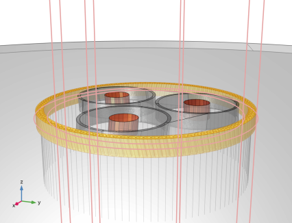
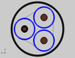
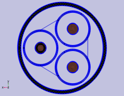
In the Model Builder window, expand the Component 1 (comp1) > Geometry 1 node, then click Phases and Screens (wp1).
2
In the Settings window for Work Plane, type Phases, Screens, and Sea Bed in the Label text field.
3
Click  Build Selected.
Phases, Screens, and Sea Bed (wp1) > Convert to Solid 1 (csol1)
1
In the Model Builder window, expand the Component 1 (comp1) > Geometry 1 > Phases, Screens, and Sea Bed (wp1) > Plane Geometry node, then click Convert to Solid 1 (csol1).
2
Right-click Convert to Solid 1 (csol1) and choose Delete.
Phases, Screens, and Sea Bed (wp1) > Circle 2 (c2)
1
In the Work Plane toolbar, click  Circle.
2
In the Settings window for Circle, locate the Size and Shape section.
3
In the Radius text field, type 5*Dcab/2.
4
In the Work Plane toolbar, click  Build All.
5
Click the  Zoom Extents button in the Graphics toolbar.
The circle that marks the outer perimeter of the model is moved to the work plane Phases, Screens, and Sea Bed (wp1), to allow the sea bed to twist together with the phases and the screens. The conversion step Convert to Solid 1 (csol1) is removed, because the circle makes it obsolete.
Cable Armor
1
In the Model Builder window, under Component 1 (comp1) > Geometry 1 click Cable Armor and Sea Bed (wp2).
2
In the Settings window for Work Plane, type Cable Armor in the Label text field.
3
Click  Build Selected.
Cable Armor (wp2) > Circle 1 (c1)
In the Model Builder window, under Component 1 (comp1) > Geometry 1 > Cable Armor (wp2) > Plane Geometry right-click Circle 1 (c1) and choose Delete.
Cable Armor (wp2) > Convert to Solid 1 (csol1)
1
In the Work Plane toolbar, click  Conversions and choose Convert to Solid.
2
Click in the Graphics window and then press Ctrl+A to select all objects.
3
In the Work Plane toolbar, click  Build All.
4
Click the  Zoom Extents button in the Graphics toolbar.
5
Click the Zoom In button in the Graphics toolbar, twice.
Here, the circle that forms the exterior boundaries is removed. A new conversion step Convert to Solid 1 (csol1) is added, to make sure the shape is extruded properly by the sweep operation Sweep 2 (swe2).
Now, continue by adding some more mesh control entities, to ensure that the mesh is the same for each armor wire.
Mesh Control Entities (wp3)
1
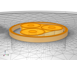
In the Model Builder window, under Component 1 (comp1) > Geometry 1 click Mesh Control Entities (wp3).
2
In the Settings window for Work Plane, click  Build Selected.
Mesh Control Entities (wp3) > Plane Geometry
In the Model Builder window, expand the Mesh Control Entities (wp3) node, then click Plane Geometry.
Mesh Control Entities (wp3) > Line Segment 6 (ls6)
1
In the Work Plane toolbar, click  More Primitives and choose Line Segment.
2
In the Settings window for Line Segment, locate the Starting Point section.
3
From the Specify list, choose Coordinates.
4
In the xw text field, type Darm/2-2*Tarm/3.
5
Locate the Endpoint section. Click to select the  Activate Selection toggle button for End vertex.
6
7
On the object sca3(35), select Point 5 only.
8
Click  Build Selected.
Mesh Control Entities (wp3) > Line Segment 7 (ls7)
1
In the Work Plane toolbar, click  More Primitives and choose Line Segment.
2
In the Settings window for Line Segment, locate the Starting Point section.
3
From the Specify list, choose Coordinates.
4
In the xw text field, type Darm/2+2*Tarm/3.
5
Locate the Endpoint section. Click to select the  Activate Selection toggle button for End vertex (if not activated already).
6
On the object sca3(39), select Point 5 only.
7
Click  Build Selected.
Mesh Control Entities (wp3) > Rotate 8 (rot8)
1
In the Work Plane toolbar, click  Transforms and choose Rotate.
2
Select the objects ls6 and ls7 only.
3
In the Settings window for Rotate, locate the Rotation section.
4
In the Angle text field, type 360[deg]*range(1/Narm,1/Narm,1).
5
In the Work Plane toolbar, click  Build All.
6
Click the  Zoom Extents button in the Graphics toolbar.
7
Click the  Zoom In button in the Graphics toolbar, twice.
More information on expressions such as “360[deg]*range(1/Narm,1/Narm,1)”, can be found in the Geometry & Mesh 3D tutorial.
These additions to Mesh Control Entities (wp3) will make it possible to consider the mesh on the periodicity plane in the direct vicinity of the armor wire cross section, to be a unit cell. Once a surface mesh has been constructed for one armor wire, it can be copied to all the other wires.
With the mesh in all armor wires identical, the armor wires are able to shift position while maintaining mesh conformity (that is; when comparing the source periodicity plane to the destination). This makes it possible for the periodic condition to connect the armor wires to their neighbors, rather then themselves — see section Short-Twisted Periodicity and Mesh Conformity.
In effect, the armor wires will be put in series (as is done for the 2.5D configuration): You can consider the short pieces of armor wire to be a number of series-connected sections that form one full-periodic wire (see Figure 4).
Geometry 1
1
In the Model Builder window, right-click Geometry 1 and choose Build All (this should take a couple of seconds).
2
In the Model Builder window, collapse the Component 1 (comp1) > Geometry 1 > Phases, Screens, and Sea Bed (wp1) node, the Cable Armor (wp2) node, and the Mesh Control Entities (wp3) node.
Next, the selections need to be updated. This will make the modifications in the mesh sequence a lot easier. Start by removing some selections that have become obsolete.
Definitions
Free Triangular 3
In the Model Builder window, under Component 1 (comp1) > Definitions > Selections > Mesh Selections right-click Free Triangular 3 and choose Delete.
Free Triangular 3, Size 1
Right-click Free Triangular 3, Size 1 and choose Delete.
Convert 1
In the Model Builder window, right-click Convert 1 and choose Delete.
Now, continue by updating one of the selections for the swept mesh, and add some new selections for the mesh in the armor.
Swept 1, Distribution 2
1
In the Model Builder window, under Component 1 (comp1) > Definitions > Selections > Mesh Selections click Swept 1, Distribution 2.
2
In the Settings window for Cylinder, locate the Size and Shape section.
3
In the Outer radius text field, type Darm/2+Tarm.
Copy Face 4
1
In the Definitions toolbar, click  Cylinder.
2
In the Settings window for Cylinder, type Copy Face 4 in the Label text field.
3
Locate the Geometric Entity Level section. From the Level list, choose Boundary.
4
Locate the Input Entities section. From the Entities list, choose From selections.
5
Under Selections, click  Add.
6
In the Add dialog, select Not Armor, Boundaries Bottom in the Selections list.
7
8
In the Settings window for Cylinder, locate the Size and Shape section.
9
In the Outer radius text field, type Darm/2.
10
In the Inner radius text field, type Darm/2-Tarm.
11
Locate the Output Entities section. From the Include entity if list, choose All vertices inside cylinder.
12
In the Graphics window toolbar, clicknext to  Go to Default View, then choose Go to View 3 (Orthographic, Bottom).
Copy Face 5
1
Right-click Copy Face 4 and choose Duplicate.
2
In the Settings window for Cylinder, type Copy Face 5 in the Label text field.
3
Locate the Size and Shape section. In the Outer radius text field, type Darm/2+Tarm.
4
In the Inner radius text field, type Darm/2.
Free Triangular 3
1
In the Definitions toolbar, click  Cylinder.
2
In the Settings window for Cylinder, type Free Triangular 3 in the Label text field.
3
Locate the Geometric Entity Level section. From the Level list, choose Boundary.
4
Locate the Input Entities section. From the Entities list, choose From selections.
5
Under Selections, click  Add.
6
In the Add dialog, in the Selections list, choose Copy Face 4 and Copy Face 5.
7
8
In the Settings window for Cylinder, locate the Size and Shape section.
9
In the Outer radius text field, type Tarm.
10
Locate the Position section. In the x text field, type Darm/2.
11
In the y text field, type Tarm/2.
12
Locate the Output Entities section. From the Include entity if list, choose All vertices inside cylinder.
13
Click the Zoom to Selection button in the Graphics toolbar.
14
Click the Zoom Out button in the Graphics toolbar, twice.
Copy Face 4, Source Boundaries
1
In the Definitions toolbar, click  Intersection.
2
In the Settings window for Intersection, type Copy Face 4, Source Boundaries in the Label text field.
3
Locate the Geometric Entity Level section. From the Level list, choose Boundary.
4
Locate the Input Entities section. Under Selections to intersect, click  Add.
5
In the Add dialog, in the Selections to intersect list, choose Copy Face 4 and Free Triangular 3.
6
Copy Face 4, Destination Boundaries
1
In the Definitions toolbar, click  Difference.
2
In the Settings window for Difference, type Copy Face 4, Destination Boundaries in the Label text field.
3
Locate the Geometric Entity Level section. From the Level list, choose Boundary.
4
Locate the Input Entities section. Under Selections to add, click  Add.
5
In the Add dialog, select Copy Face 4 in the Selections to add list.
6
7
In the Settings window for Difference, locate the Input Entities section.
8
Under Selections to subtract, click  Add.
9
In the Add dialog, select Copy Face 4, Source Boundaries in the Selections to subtract list.
10
11
Click the Zoom to Selection button in the Graphics toolbar.
Copy Face 5, Source Boundaries
1
In the Definitions toolbar, click  Intersection.
2
In the Settings window for Intersection, type Copy Face 5, Source Boundaries in the Label text field.
3
Locate the Geometric Entity Level section. From the Level list, choose Boundary.
4
Locate the Input Entities section. Under Selections to intersect, click  Add.
5
In the Add dialog, in the Selections to intersect list, choose Copy Face 5 and Free Triangular 3.
6
7
Click the Zoom to Selection button in the Graphics toolbar.
8
Click the Zoom Out button in the Graphics toolbar, twice.
Copy Face 5, Destination Boundaries
1
In the Definitions toolbar, click  Difference.
2
In the Settings window for Difference, type Copy Face 5, Destination Boundaries in the Label text field.
3
Locate the Geometric Entity Level section. From the Level list, choose Boundary.
4
Locate the Input Entities section. Under Selections to add, click  Add.
5
In the Add dialog, select Copy Face 5 in the Selections to add list.
6
7
In the Settings window for Difference, locate the Input Entities section.
8
Under Selections to subtract, click  Add.
9
In the Add dialog, select Copy Face 5, Source Boundaries in the Selections to subtract list.
10
11
Click the Zoom to Selection button in the Graphics toolbar.
Free Triangular 4
1
In the Definitions toolbar, click  Difference.
2
In the Settings window for Difference, type Free Triangular 4 in the Label text field.
3
Locate the Geometric Entity Level section. From the Level list, choose Boundary.
4
Locate the Input Entities section. Under Selections to add, click  Add.
5
In the Add dialog, select Cross Section, Bottom in the Selections to add list.
6
7
In the Settings window for Difference, locate the Input Entities section.
8
Under Selections to subtract, click  Add.
9
In the Add dialog, in the Selections to subtract list, choose Phases, Boundaries Bottom, Screens, Boundaries Bottom (Mapped 3), Armor, Boundaries Bottom, Mapped 4, Copy Face 4, and Copy Face 5.
10
11
In the Model Builder window, collapse the Component 1 (comp1) > Definitions > Selections node.
Organizing your selections like this may seem a bit of a hassle at first glance. After all; you could just click on the boundaries in the graphics window and obtain your selections that way. On the long term, however, this may save you a lot of time: You can change your geometric parameters all you like, remove and rebuild your geometry entirely, or even switch to a CAD-imported geometry, while still keeping your selections intact. Also, some of these selections contain over a hundred entities. Selecting those by hand can be tedious and error-prone.
Mesh 1
Now, before solving, the mesh sequence will have to be modified to ensure conforming meshes. In addition to this, the mesh will be refined a bit to better resolve the solution close to the armor wires (now that the length of the model has been reduced a hundredfold, you can afford some additional refinement).
Size 1
1
In the Model Builder window, expand the Component 1 (comp1) > Mesh 1 > Mapped 3 node, then click Size 1.
2
In the Settings window for Size, locate the Element Size Parameters section.
3
In the Maximum element size text field, type 2*Tpbs.
4
In the Minimum element size text field, type 2*Tpbs.
5
Click  Build Selected.
Free Triangular 3
1
In the Model Builder window, under Component 1 (comp1) > Mesh 1 click Free Triangular 3.
2
In the Settings window for Free Triangular, locate the Boundary Selection section.
3
From the Selection list, choose Free Triangular 3.
4
Click the Zoom to Selection button in the Graphics toolbar.
5
Click the Zoom Out button in the Graphics toolbar, twice.
Size 1
1
In the Model Builder window, expand the Free Triangular 3 node, then click Size 1.
2
In the Settings window for Size, locate the Geometric Entity Selection section.
3
From the Selection list, choose Free Triangular 3.
4
Locate the Element Size Parameters section. Clear the Maximum element growth rate checkbox.
5
Click  Build Selected.
Copy Face 4
1
In the Mesh toolbar, click  Copy and choose Copy Face.
2
In the Settings window for Copy Face, locate the Source Boundaries section.
3
From the Selection list, choose Copy Face 4, Source Boundaries.
4
Locate the Destination Boundaries section. Click to select the  Activate Selection toggle button.
5
From the Selection list, choose Copy Face 4, Destination Boundaries.
6
Click  Build Selected.
7
Click the Zoom to Selection button in the Graphics toolbar.
Copy Face 5
1
In the Mesh toolbar, click  Copy and choose Copy Face.
2
In the Settings window for Copy Face, locate the Source Boundaries section.
3
From the Selection list, choose Copy Face 5, Source Boundaries.
4
Click the Zoom to Selection button in the Graphics toolbar.
5
Click the Zoom Out button in the Graphics toolbar, twice.
6
Locate the Destination Boundaries section. Click to select the  Activate Selection toggle button.
7
From the Selection list, choose Copy Face 5, Destination Boundaries.
8
Click  Build Selected.
9
Click the Zoom to Selection button in the Graphics toolbar.
Mapped 4
1
In the Model Builder window, right-click Mapped 4 and choose Build Selected.
As you can see in this close-up, the mesh is identical for all armor wire cross sections and their neighboring surfaces. The mesh quality close to the armor has been improved significantly (compared to the long-periodic model).
Free Triangular 4
1
In the Mesh toolbar, click  More Generators and choose Free Triangular.
2
In the Settings window for Free Triangular, locate the Boundary Selection section.
3
From the Selection list, choose Free Triangular 4.
Size 1
1
Right-click Free Triangular 4 and choose Size.
2
In the Settings window for Size, locate the Element Size section.
3
Click the Custom button.
4
Locate the Element Size Parameters section.
5
Select the Minimum element size checkbox. In the associated text field, type Tarm.
6
Select the Maximum element growth rate checkbox. In the associated text field, type 1.3.
7
Click  Build Selected.
Next, update the settings for the swept mesh, so that it uses an appropriate amount of elements in the sweep direction.
Distribution 1
1
In the Model Builder window, expand the Component 1 (comp1) > Mesh 1 > Swept 1 node, then click Distribution 1.
2
In the Settings window for Distribution, locate the Distribution section.
3
In the Number of elements text field, type 3.
Distribution 2
1
In the Model Builder window, click Distribution 2.
2
In the Settings window for Distribution, locate the Distribution section.
3
In the Number of elements text field, type 4.
Swept 1
1
In the Model Builder window, right-click Swept 1 and choose Build Selected.
2
In the Settings window for Swept, in the Graphics window toolbar, clicknext to  Go to Default View, then choose Go to View 5 (Perspective).
You have now updated the swept mesh for the phases, the screens, and the armor. The mesh conversion step Convert 1 is not required any longer: The pyramids that are added automatically as an interface between the swept mesh and the tetrahedra, will have a sufficient quality now. You can finalize the mesh by deleting the conversion step and updating Free Tetrahedral 1.
Convert 1
In the Model Builder window, right-click Convert 1 and choose Delete.
Free Tetrahedral 1
1
In the Model Builder window, under Component 1 (comp1) > Mesh 1 click Free Tetrahedral 1.
2
In the Settings window for Free Tetrahedral, click to expand the Scale Geometry section.
3
In the z-direction scale text field, type 1.
This will restore the tetrahedral mesh to become an “ordinary” isotropic mesh once again (for the long-periodic model it was stretched by a factor of six in the z direction, to save degrees of freedom).
Size 1
1
In the Model Builder window, expand the Free Tetrahedral 1 node, then click Size 1.
2
In the Settings window for Size, locate the Element Size Parameters section.
3
In the Maximum element growth rate text field, type 1.3.
4
Click  Build All (this should take a couple of seconds).
5
In the Model Builder window, collapse the Mesh 1 node.
6
Right-click Component 1 (comp1) > Mesh 1 and choose Statistics.
7
In the Settings window for Mesh, check the following statistics:
The actual numbers you get will probably deviate (by less than a percent), and will depend on your operating system, COMSOL version, and geometry representation — COMSOL kernel, or CAD kernel.
Study 1
The short-periodic configuration tends to cause small numbers on the matrix diagonal. Therefore, it is better to use a direct solver with pivoting enabled. This may consume more memory (and perhaps it will iterate a couple of times before it has allocated the appropriate amount of RAM), but the solver will be more stable. Now that the number of degrees of freedom has been reduced drastically, it is better to go for stability rather than a memory-lean solver configuration.
Let us switch to a different solver and then compute.
Solution 1 (sol1)
1
In the Model Builder window, expand the Study 1 > Solver Configurations > Solution 1 (sol1) > Stationary Solver 2 node, then click Suggested Direct Solver (mf).
2
In the Settings window for Direct, locate the General section.
3
From the Solver list, choose MUMPS.
4
In the Study toolbar, click  Compute (this should take a minute or so).
Results
Magnetic Flux Density, z-Component Norm (mf)
Compared to the long-periodic model the plot shows only a thin slice of cable, but the field distribution should still be the same.
Next, you can verify that the results indeed correspond to those from the model stored as submarine_cable_08_c_inductive_effects_3d.mph.
Phase Losses
1
In the Model Builder window, expand the Results > Derived Values node, then click Phase Losses.
2
In the Settings window for Volume Integration, locate the Expressions section.
3
In the table, update the description. Type Phase losses (linres 3D, short-periodic), that is; replace “linres 3D” with “linres 3D, short-periodic”.
4
In the Settings window for Volume Integration, click Evaluate.
Screen Losses, Armor Losses, Phase AC Resistance, and Phase Inductance
Repeat these steps for Screen Losses, Armor Losses, Phase AC Resistance, and Phase Inductance.
Table
1
Go to the Table window.
The losses per kilometer should be about 59 kW, 14.7 kW, and 2.8 kW for the phases, the screens, and the armor respectively. These values are effectively the same as those from the long-periodic model (see the previous table column), with a deviation of about 0.1–0.4% for the phases and the screens. This lies well within the expected accuracy for these models.
For the armor, the deviation is a bit larger (about 1–2%), since the mesh close to the armor has been refined. If you evaluate the resistive- and magnetic losses in the armor separately (using the expressions mf.Qrh and mf.Qml), you will see the magnetic losses still make up about 76% of the total armor losses.
The phase AC resistance is still 59 mΩ/km, and the inductance is still 0.45 mH/km; they deviate from their previous values by about 0.1–0.4%.
So, for all intends and purposes, this model produces precisely the same output as the long one for only a fraction of the computational effort! 
In order to finalize the model, check the plots and modify them a bit so that they look good with the short geometry.
Mesh Quality, Volume Elements
1
In the Model Builder window, under Results click Mesh Quality, Volume Elements.
2
In the Settings window for 3D Plot Group, locate the Plot Settings section.
3
From the View list, choose View 2 (Orthographic, Top).
Mesh 1
1
In the Model Builder window, expand the Mesh Quality, Volume Elements node, then click Mesh 1.
2
In the Settings window for Mesh, click to expand the Element Filter section.
3
Clear the Enable filter checkbox.
4
In the Mesh Quality, Volume Elements toolbar, click  Plot.
5
Click the  Transparency button in the Graphics toolbar once (to disable it).
Mesh 1
1
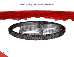
In the Model Builder window, expand the Results > Mesh Quality, Poor Quality Elements node, then click Mesh 1.
2
In the Settings window for Mesh, locate the Coloring and Style section.
3
From the Wireframe color list, choose Black.
4
Locate the Element Filter section. Clear the Enable filter checkbox.
5
In the Mesh Quality, Poor Quality Elements toolbar, click  Plot.
Mesh Comparison, Source and Destination
1
In the Model Builder window, under Results click Mesh Comparison, Source and Destination.
2
In the Mesh Comparison, Source and Destination toolbar, click  Plot.
This plot is of particular importance for checking mesh conformity. For more on how and why this plot is constructed, see the Geometry & Mesh 3D tutorial.
Cut Plane 3
1
In the Model Builder window, expand the Results > Datasets node, then click Cut Plane 3.
2
In the Settings window for Cut Plane, locate the Plane Data section.
3
In the z-coordinate text field, type -Lsec/2.
4
In the Distances text field, type Lsec.
5
Magnetic Flux Density, z-Component Norm (mf)
1
In the Model Builder window, under Results click Magnetic Flux Density, z-Component Norm (mf).
2
In the Magnetic Flux Density, z-Component Norm (mf) toolbar, click  Plot.
Longitudinal Current Density (mf)
1
In the Model Builder window, click Longitudinal Current Density (mf).
2
In the Longitudinal Current Density (mf) toolbar, click  Plot.
Transverse Current Density (mf)
1
In the Model Builder window, click Transverse Current Density (mf).
2
In the Transverse Current Density (mf) toolbar, click  Plot.
Longitudinal and Transverse Current Density (mf)
1
In the Model Builder window, click Longitudinal and Transverse Current Density (mf).
2
In the Longitudinal and Transverse Current Density (mf) toolbar, click  Plot.
3
Click the  Go to Default View button in the Graphics toolbar.
For more information on the details of these plots, see section Modeling Instructions (including Modeling Instructions Extruded 2D Model) and section Modeling Instructions — 3D Twist Model.
Volumetric Loss Density, Electromagnetic (mf)
1
In the Model Builder window, click Volumetric Loss Density, Electromagnetic (mf).
2
In the Volumetric Loss Density, Electromagnetic (mf) toolbar, click  Plot.
The armor loss shows the same spatial distribution as the one discussed in section Modeling Instructions — Linearized Resistivity 3D: Trails of loss concentration are spiraling around the cable’s axis. In this case it is not as easy to see, but the spiral will emerge when you start stacking slices like this one, and apply the twisted periodicity.
So even for three-phase cable models with a counter-twisted magnetic armor it is possible to build an accurate 3D model that solves in a minute: About the same time it takes to solve a 2D model. This is such a massive improvement compared to the statistics reported only recently in sources like reference [2], that there is really no point in trying to increase the performance much further.
Instead, twisted periodicity and short-twisted periodicity is expected to be used in the coming years to investigate more and more complicated twisting schemes — starting with a double twisted armor (see section Short-Twisted Periodicity and Double-Twisted Armors), and followed by fully resolved Milliken conductors. For the standard three-phase cable with a single twisted armor however, the search for more efficient solving strategies seems pretty much over.
You have now finished the final section of the final chapter of this tutorial series. The resulting file is available as submarine_cable_08_inductive_effects_3d.mph.
Please have a look at the previous chapters if you have not already done so. If you still have any questions about cable modeling in COMSOL Multiphysics, feel free to contact your local COMSOL sales team, or write to COMSOL Support if your license supports it.
From the File menu, choose Save.

1
They are typically based on IEC 60287 [1] or similar standards.

2
Notice that initially, James Clerk Maxwell did not include the displacement currents, leading to a law that is valid under stationary conditions only (known as Ampère’s circuital law). He added the displacement currents a couple of years later — at equation (112) in his 1861 paper “On Physical Lines of Force” — resulting in what is now referred to as “Maxwell–Ampère’s law” (or, less formally; “Ampère’s law”).

3
Since this model runs in the frequency domain, you are restricted to linear material properties. It is possible to approximate the effect of a nonlinear material though; using effective nonlinear magnetic curves. For more on this, check the AC/DC Module User’s Guide.

4
This phenomenon leads to gauge freedom. For more info, see the AC/DC Module User’s Guide.

5
Notice that, with the electric field being defined solely in terms of the magnetic vector potential, we have been excluding the electric scalar potential, that is; V = 0 everywhere. This choice is known as the Weyl or Hamiltonian gauge. For more information about different gauges and gauge fixing, see the AC/DC Module User’s Guide.

6
For more, see the COMSOL Multiphysics Reference Manual or reference [8], for example.

7
The Magnetic Fields interface only uses the magnetic vector potential A, and is therefore known as the A-formulation. The Magnetic and Electric Fields interface uses both the magnetic vector potential A, and the electric scalar potential V. This is known as the AV-formulation. The Rotating Machinery, Magnetic interface combines the magnetic vector potential A in some domains, with the magnetic scalar potential Vm in others — so; not in the same domains, at the same time — and could be considered an AVm-formulation.

8
If the cancellation were perfect, it would mean A' and A are equal. And if they are equal, there is no point in solving the model a second time. Therefore, the procedure should be seen as a first-order correction. You can iterate the process if you like, and come up with second- or third-order corrections. In practice, the first one seems more than enough.

9
Notice that, as this is COMSOL Multiphysics, the user is free to choose any relation σ(T), although not every relation will result in good convergence — or a (unique) solution for that matter. Having small or zero higher-order terms in the relation σ(T) will keep the computational effort low.

10
Note that this is the same assumption as the one used for the 2.5D models in the Inductive Effects tutorial.

11
Notice that in the frequency domain the total loss Qtot and the AC resistance Rac are tied to each other, through Qtot = |I |2Rac/2. Since energy needs to be conserved, an increase in one means an increase in the other (see the Thermal Effects tutorial).

12
It may not work for all cable designs however, validation will remain important.

13
Strictly speaking, stationary-electric reasoning is not applicable. It is done here, to give an “intuitive” explanation. The correct value for the resistance in the frequency domain, is the AC resistance Rac. That one reflects all losses in the cable, including those in the screens and armor: Qtot = |I |2Rac/2.

14
These results can be validated by testing different values for the stabilizing conductivity and extrapolating the results to the point where the stabilizing conductivity becomes zero.