PDF

Small-Signal Analysis of an Inductor
Introduction
This example uses the model Inductor in an Amplifier Circuit from the AC/DC Module Application Library without the circuits definition. This model consists of an inductor with a nonlinear magnetic core that shows a changing inductance when the current increases. In this example, you investigate the small-signal inductance as a function of current through the inductor.
For the correct evaluation of small-signal lumped parameters like electric impedance and inductance, understanding the lindev operator is mandatory. Please consult the section on Small-Signal Analysis, Prestressed Analysis, and Harmonic Perturbation Plot Settings in the COMSOL Multiphysics Reference Manual.
Application Library path: ACDC_Module/Devices,_Inductive/small_signal_analysis_of_inductor
Modeling Instructions
From the File menu, choose New.
New
In the New window, click  Model Wizard.
Model Wizard
1
In the Model Wizard window, click  2D Axisymmetric.
2
In the Select Physics tree, select AC/DC > Electromagnetic Fields > Magnetic Fields (mf).
3
Click Add.
4
Click  Study.
5
In the Select Study tree, select Preset Studies for Selected Physics Interfaces > Small-Signal Analysis, Frequency Domain.
6
Global Definitions
Import the model parameters from a text file.
Parameters 1
1
In the Model Builder window, under Global Definitions click Parameters 1.
2
In the Settings window for Parameters, locate the Parameters section.
3
Click  Load from File.
4
Geometry 1
Circle 1 (c1)
1
In the Geometry toolbar, click  Circle.
2
In the Settings window for Circle, locate the Size and Shape section.
3
In the Radius text field, type dr.
4
In the Sector angle text field, type 180.
5
Locate the Rotation Angle section. In the Rotation text field, type -90.
6
Click  Build Selected.
Rectangle 1 (r1)
1
In the Geometry toolbar, click  Rectangle.
2
In the Settings window for Rectangle, locate the Size and Shape section.
3
In the Width text field, type 3*cr.
4
In the Height text field, type il*1.5.
5
Locate the Position section. In the z text field, type -il*1.5/2.
6
Right-click Rectangle 1 (r1) and choose Build Selected.
Rectangle 2 (r2)
1
In the Geometry toolbar, click  Rectangle.
2
In the Settings window for Rectangle, locate the Size and Shape section.
3
In the Width text field, type coor-coir.
4
In the Height text field, type il.
5
Locate the Position section. In the r text field, type coir.
6
In the z text field, type -il/2.
7
Right-click Rectangle 2 (r2) and choose Build Selected.
Rectangle 3 (r3)
1
In the Geometry toolbar, click  Rectangle.
2
In the Settings window for Rectangle, locate the Size and Shape section.
3
In the Width text field, type (coor-coir)*2.
4
In the Height text field, type il*1.1.
5
Locate the Position section. In the r text field, type coir*0.8.
6
In the z text field, type -il/2*1.1.
7
Right-click Rectangle 3 (r3) and choose Build Selected.
Fillet 1 (fil1)
1
In the Geometry toolbar, click  Fillet.
Next, select all ten points in the internal of the geometry as follows:
2
Click the Select Box button in the Graphics toolbar.
3
4
In the Settings window for Fillet, locate the Radius section.
5
In the Radius text field, type fr.
6
Click  Build All Objects.
The geometry is now complete.
Magnetic Fields (mf)
The nonlinear inductor must use a different constitutive relation for the magnetic field. Thus a separate Ampère’s Law feature must be entered for this.
Nonlinear Core
1
In the Physics toolbar, click  Domains and choose Ampère’s Law in Solids.
2
In the Settings window for Ampère’s Law in Solids, type Nonlinear Core in the Label text field.
3
4
Locate the Constitutive Relation B-H section. From the Magnetization model list, choose B-H curve.
5
Locate the Constitutive Relation Jc-E section. From the σ list, choose User defined. In the associated text field, type 1000.
Usually, a laminated core is used to decrease the eddy current loss. Here, set a user defined conductivity to simulate such an effect.
Define the coil with the static excitation.
Domain Coil 1
1
In the Physics toolbar, click  Domains and choose Domain Coil.
2
3
In the Settings window for Domain Coil, locate the Coil section.
4
In the Coil name text field, type coil.
5
From the Conductor model list, choose Homogenized multiturn.
6
Locate the Homogenized Conductor section. In the N text field, type cn.
7
In the σ text field, type csigma.
8
From the Coil wire cross-section area list, choose User defined.
9
Find the High-frequency effective loss subsection. Clear the Include harmonic loss checkbox.
10
In the a text field, type cwc.
11
Locate the Coil section. In the Icoil text field, type cIdc.
Add the time-harmonic excitation.
Harmonic Perturbation 1
1
In the Physics toolbar, click  Attributes and choose Harmonic Perturbation.
2
In the Settings window for Harmonic Perturbation, locate the Harmonic Perturbation section.
3
In the Icoil text field, type cIac.
Add Material
1
In the Materials toolbar, click  Add Material to open the Add Material window.
2
Go to the Add Material window.
3
In the tree, select Built-in > Copper.
4
Click the Add to Component button in the window toolbar.
5
In the tree, select Nonlinear Magnetic > Low Carbon Steel > Low Carbon Steel 1006.
6
Click the Add to Component button in the window toolbar.
7
In the Materials toolbar, click  Add Material to close the Add Material window.
Materials
Copper (mat1)
Select Domain 4 only.
Low Carbon Steel 1006 (mat2)
1
In the Model Builder window, click Low Carbon Steel 1006 (mat2).
2
Definitions
Define a scalar variable based on the ratio between magnetic flux density and magnetic field. The variable can be interpreted as the relative permeability in a linear material or for small field strength. Plotting this variable is useful to visualize the saturation status of the iron core.
Variables 1
1
In the Definitions toolbar, click  Local Variables.
2
In the Settings window for Variables, locate the Variables section.
3
The stationary solver will sweep the value of the parameter cIdc (DC bias current) over a range from 1 mA to 50 mA. The stationary solution computed at each point will be used as linearization point for the corresponding frequency-domain perturbation step. Thus you need to set up a continuation sweep in the stationary solver.
Study 1
Step 1: Stationary
1
In the Model Builder window, under Study 1 click Step 1: Stationary.
2
In the Settings window for Stationary, click to expand the Study Extensions section.
3
Select the Auxiliary sweep checkbox.
4
5
Step 2: Frequency-Domain Perturbation
1
In the Model Builder window, click Step 2: Frequency-Domain Perturbation.
2
In the Settings window for Frequency-Domain Perturbation, locate the Study Settings section.
3
From the Frequency unit list, choose kHz.
4
In the Frequencies text field, type f0.
Apply to the frequency-domain solver the same sweep that was applied to the stationary solver. This ensures that the stationary parameter (the DC current) is recognized properly.
5
Click to expand the Study Extensions section. Select the Auxiliary sweep checkbox.
6
7
Solution stability benefits from tightening the nonlinear tolerance for the stationary step.
Solution 1 (sol1)
In the Study toolbar, click  Show Default Solver.
Step 1: Stationary
1
In the Model Builder window, under Study 1 click Step 1: Stationary.
2
In the Settings window for Stationary, locate the Study Settings section.
3
From the Tolerance list, choose User controlled.
4
In the Relative tolerance text field, type 1e-6.
5
In the Study toolbar, click  Compute.
Results
Coil Inductance
1
In the Results toolbar, click  1D Plot Group.
2
In the Settings window for 1D Plot Group, type Coil Inductance in the Label text field.
Global 1
1
Right-click Coil Inductance and choose Global.
2
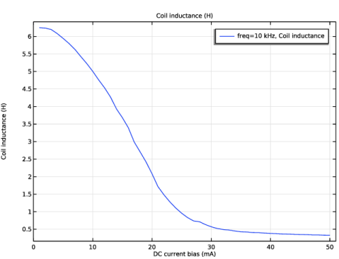
In the Settings window for Global, click Replace Expression in the upper-right corner of the y-Axis Data section. From the menu, choose Component 1 (comp1) > Magnetic Fields > Coil parameters > mf.LCoil_coil - Coil inductance - H.
The Global Plot can be used to plot physical quantities from the stationary solution, from the harmonic perturbation solution, or in other cases available in the Expression evaluated for list. The Compute differential checkbox is used to compute the differential of the physical quantity around the linearization point. In the case of lumped parameters, the differential should not be computed, since they are defined as the ratio of two differentials. Leave that option unchecked.
3
Locate the x-Axis Data section. From the Parameter list, choose Expression.
4
In the Expression text field, type cIdc.
5
From the Unit list, choose mA.
6
In the Coil Inductance toolbar, click  Plot.
The plot will show the inductance of the component at different values of the bias currents.The inductance drops significantly as a consequence of the saturation of the core. The saturation can be visualized by plotting the relative permeability of the iron core.
The small signal inductance is plotted versus the DC bias current.
Surface 1
1
In the Model Builder window, expand the Magnetic Flux Density (mf) node, then click Surface 1.
2
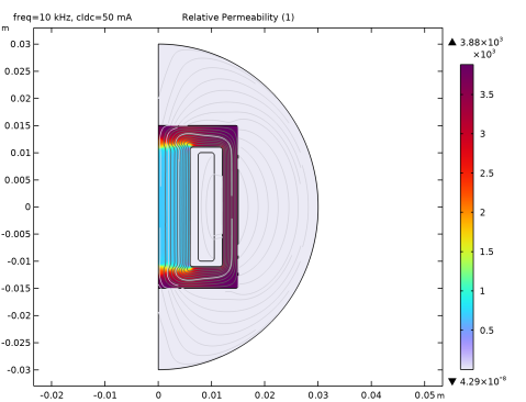
In the Settings window for Surface, click Replace Expression in the upper-right corner of the Expression section. From the menu, choose Component 1 (comp1) > Definitions > Variables > mur - Relative Permeability - 1.
3
Locate the Expression section. From the Expression evaluated for list, choose Static solution.
4
In the Magnetic Flux Density (mf) toolbar, click  Plot.
The plot shows that the relative permeability of the inner core has dropped well below the value at zero field of 3882.
The Harmonic Perturbation subfeature can be added to a wide range of source features in the AC/DC Module. A linear perturbation study can be manually performed on any other source by using the linper operator as shown next.
Magnetic Fields (mf)
Domain Coil 1
1
In the Model Builder window, under Component 1 (comp1) > Magnetic Fields (mf) click Domain Coil 1.
2
In the Settings window for Domain Coil, locate the Coil section.
3
In the Icoil text field, type cIdc + linper(cIac).
Harmonic Perturbation 1
In the Model Builder window, right-click Harmonic Perturbation 1 and choose Disable.
Study 1
In the Study toolbar, click  Compute.
Results
Magnetic Flux Density (mf)
Inspect the results again and confirm they did not change.