|
|
|
|
•
|
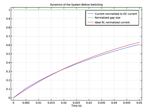
Before plunger motion: Figure 7 shows the first stage of the simulation, when the spring is not yet compressed. Blue and green lines represent normalized currents and gap size respectively. Red line is an exponential fit for the RL current dynamics of the initially nonmoving inductor — the response of an ideal system.
|
|
•
|
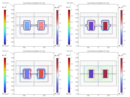
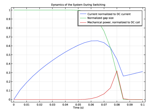
During plunger motion: the compression of the spring and the resulting closure of the gap are visualized in Figure 8. Normalized currents and gap size are represented by blue and green lines respectively, the red line showing instead the mechanical power (which is nonzero only during the motion of the plunger).
|
|
•
|
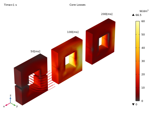
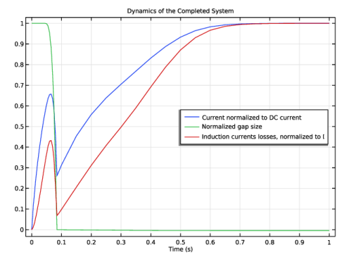
After plunger motion: Figure 9 refers to the last stage of simulation, when the spring is completely compressed. The red line shows the induction losses in the core, which are significant during the movement of the plunger. Depending on the details of the device and the desired performance, this aspect may need to be taken into account during the design process. After the movement is completed, the current starts increasing again as expected in a (nonlinear) RL circuit.
 |
|
1
|
|
2
|
|
3
|
Click Add.
|
|
4
|
|
5
|
Click Add.
|
|
6
|
Click
|
|
7
|
In the Select Study tree, select Preset Studies for Some Physics Interfaces > Coil Geometry Analysis.
|
|
8
|
Click
|
|
1
|
|
2
|
|
3
|
Click
|
|
4
|
Browse to the model’s Application Libraries folder and double-click the file power_switch_multibody_parameters.txt.
|
|
1
|
|
2
|
|
1
|
|
2
|
|
3
|
|
4
|
|
5
|
|
1
|
|
2
|
|
3
|
|
4
|
|
5
|
|
6
|
|
1
|
|
2
|
Select the object r1 only.
|
|
3
|
|
4
|
|
5
|
Select the object r2 only.
|
|
1
|
|
2
|
|
3
|
|
4
|
|
5
|
|
6
|
Select the object dif1 only.
|
|
7
|
|
8
|
Click
|
|
9
|
|
1
|
In the Model Builder window, under Global Definitions right-click Geometry Parts and choose 2D Part.
|
|
2
|
|
1
|
|
2
|
|
3
|
|
4
|
|
5
|
|
1
|
|
2
|
|
3
|
|
4
|
|
5
|
|
6
|
|
7
|
Click to expand the Layers section. In the table, enter the following settings:
|
|
1
|
|
2
|
|
3
|
|
4
|
|
5
|
|
1
|
|
2
|
|
3
|
|
4
|
On the object c1, select Domain 1 only.
|
|
5
|
Click
|
|
6
|
|
1
|
In the Model Builder window, under Global Definitions right-click Geometry Parts and choose 3D Part.
|
|
2
|
|
1
|
|
2
|
|
3
|
|
1
|
In the Model Builder window, under Global Definitions > Geometry Parts > Solid Parts right-click Work Plane 1 (wp1) and choose Extrude.
|
|
2
|
|
3
|
Locate the Selections of Resulting Entities section. Select the Resulting objects selection checkbox.
|
|
4
|
|
5
|
Locate the Distances section. In the table, enter the following settings:
|
|
6
|
Select the Reverse direction checkbox.
|
|
1
|
|
2
|
|
3
|
On the object ext1, select Domain 2 only.
|
|
1
|
|
2
|
|
3
|
|
1
|
In the Model Builder window, under Global Definitions > Geometry Parts > Solid Parts right-click Work Plane 2 (wp2) and choose Extrude.
|
|
2
|
|
3
|
Locate the Selections of Resulting Entities section. Select the Resulting objects selection checkbox.
|
|
4
|
|
5
|
Locate the Distances section. In the table, enter the following settings:
|
|
6
|
|
7
|
|
1
|
|
2
|
|
4
|
Click
|
|
1
|
|
2
|
|
3
|
|
4
|
|
5
|
|
6
|
|
1
|
|
2
|
Click in the Graphics window and then press Ctrl+A to select all objects.
|
|
3
|
|
1
|
|
2
|
On the object uni1, select Domain 1 only.
|
|
3
|
|
4
|
|
5
|
|
6
|
|
1
|
|
2
|
|
3
|
|
4
|
On the object pard1, select Point 34 only.
|
|
5
|
Click to expand the Local Coordinate System section. From the Origin list, choose Vertex projection.
|
|
6
|
On the object pard1, select Point 34 only.
|
|
1
|
|
2
|
|
3
|
|
4
|
On the object cro1, select Domains 1–4 only.
|
|
5
|
Click
|
|
1
|
|
2
|
|
3
|
|
4
|
|
5
|
Clear the Keep input objects checkbox.
|
|
6
|
|
1
|
|
2
|
|
3
|
|
4
|
Locate the Coordinates section. In the table, enter the following settings:
|
|
5
|
|
1
|
|
2
|
|
3
|
|
4
|
|
5
|
On the object pard1, select Point 11 only.
|
|
6
|
Click
|
|
1
|
|
2
|
|
1
|
|
2
|
|
3
|
|
4
|
|
5
|
|
1
|
|
2
|
|
3
|
|
4
|
Click
|
|
5
|
|
1
|
|
2
|
|
3
|
|
4
|
In the Add dialog, in the Selections to add list, choose Upper Core (Solid Parts 1) and Cylinder Selection 1.
|
|
5
|
|
1
|
|
2
|
|
3
|
|
1
|
|
2
|
|
3
|
|
4
|
|
5
|
|
1
|
|
2
|
|
1
|
|
2
|
|
3
|
|
4
|
|
5
|
Click OK.
|
|
6
|
|
7
|
|
8
|
|
9
|
|
1
|
|
2
|
In the Settings window for Adjacent, type Ext. boundaries to Deformed Domains in the Label text field.
|
|
3
|
|
4
|
|
5
|
|
1
|
|
2
|
|
3
|
|
4
|
|
5
|
|
1
|
|
2
|
|
3
|
|
4
|
|
5
|
|
1
|
|
2
|
|
3
|
|
4
|
|
5
|
In the Add dialog, in the Selections to intersect list, choose Ext. boundaries to Deformed Domains and Ext. Boundaries to Fixed Domains.
|
|
6
|
|
1
|
|
2
|
|
3
|
|
1
|
|
2
|
|
3
|
|
4
|
|
5
|
In the Add dialog, in the Selections to add list, choose Fixed Boundaries at Plunger and Top boundary.
|
|
6
|
|
1
|
|
2
|
|
3
|
|
4
|
|
5
|
In the Add dialog, in the Selections to intersect list, choose Ext. boundaries to Deformed Domains and Ext. Boundaries to Plunger.
|
|
6
|
|
1
|
|
2
|
|
3
|
|
4
|
Select the Group by continuous tangent checkbox.
|
|
1
|
|
2
|
|
3
|
|
4
|
|
5
|
|
1
|
|
2
|
|
3
|
|
4
|
|
5
|
|
6
|
|
7
|
Click OK.
|
|
8
|
|
9
|
|
10
|
|
11
|
|
1
|
|
2
|
Go to the Add Material window.
|
|
3
|
|
4
|
Click the Add to Component button in the window toolbar.
|
|
5
|
|
6
|
Right-click and choose Add to Component 1 (comp1).
|
|
7
|
|
1
|
|
2
|
Locate the Geometric Entity Selection section. From the Selection list, choose Coil (Solid Parts 1).
|
|
1
|
|
2
|
|
3
|
|
1
|
|
2
|
|
3
|
|
1
|
|
2
|
|
3
|
|
4
|
|
1
|
|
3
|
|
4
|
|
5
|
|
6
|
Locate the Element Size Parameters section.
|
|
7
|
|
8
|
|
1
|
|
3
|
|
4
|
|
1
|
|
1
|
|
2
|
|
3
|
|
4
|
|
1
|
|
2
|
|
3
|
|
4
|
|
5
|
|
6
|
|
7
|
|
8
|
|
1
|
|
2
|
|
3
|
|
4
|
|
1
|
|
2
|
In the Settings window for Prescribed Normal Mesh Displacement, locate the Boundary Selection section.
|
|
3
|
|
1
|
|
2
|
|
3
|
|
1
|
|
2
|
|
3
|
|
1
|
|
2
|
|
3
|
|
4
|
|
5
|
|
6
|
|
7
|
|
8
|
|
9
|
From the list, choose User defined.
|
|
10
|
|
11
|
|
1
|
In the Model Builder window, expand the Component 1 (comp1) > Magnetic Fields (mf) > Domain Coil 1 > Geometry Analysis 1 node, then click Geometry Analysis 1.
|
|
2
|
|
3
|
|
1
|
|
1
|
|
1
|
|
2
|
|
3
|
|
4
|
Locate the Domain Selection section. From the Selection list, choose Nonlinear Core (Solid Parts 1).
|
|
1
|
|
2
|
|
3
|
|
4
|
|
1
|
|
2
|
|
3
|
|
1
|
|
2
|
|
3
|
|
4
|
|
1
|
|
2
|
In the Settings window for Mass and Moment of Inertia, locate the Mass and Moment of Inertia section.
|
|
3
|
|
1
|
|
2
|
|
3
|
Specify the F vector as
|
|
1
|
|
2
|
|
3
|
|
4
|
|
5
|
|
6
|
|
1
|
|
2
|
|
3
|
|
4
|
|
5
|
|
6
|
|
1
|
In the Model Builder window, under Component 1 (comp1) right-click Definitions and choose Variables.
|
|
2
|
|
1
|
|
2
|
|
3
|
|
1
|
|
2
|
In the Settings window for Coil Geometry Analysis, locate the Physics and Variables Selection section.
|
|
3
|
In the Solve for column of the table, under Component 1 (comp1), clear the checkbox for Moving Mesh.
|
|
4
|
|
1
|
|
2
|
|
3
|
In the Settings window for 3D Plot Group, type Preprocessing: Normalized Air Gap Parameterization and Coil Direction in the Label text field.
|
|
4
|
|
5
|
|
1
|
Right-click Preprocessing: Normalized Air Gap Parameterization and Coil Direction and choose Volume.
|
|
2
|
|
3
|
|
1
|
|
2
|
|
3
|
|
4
|
|
1
|
In the Model Builder window, right-click Preprocessing: Normalized Air Gap Parameterization and Coil Direction and choose Streamline.
|
|
3
|
In the Settings window for Streamline, click Replace Expression in the upper-right corner of the Expression section. From the menu, choose Component 1 (comp1) > Magnetic Fields > Coil parameters > mf.coil1.eCoilx,...,mf.coil1.eCoilz - Coil direction (spatial frame).
|
|
4
|
Locate the Coloring and Style section. Find the Line style subsection. From the Type list, choose Tube.
|
|
5
|
|
6
|
|
7
|
|
1
|
|
2
|
Go to the Add Study window.
|
|
3
|
|
4
|
Click the Add Study button in the window toolbar.
|
|
5
|
|
1
|
|
2
|
|
3
|
|
4
|
Click to expand the Values of Dependent Variables section. Find the Values of variables not solved for subsection. From the Settings list, choose User controlled.
|
|
5
|
|
6
|
|
1
|
|
2
|
|
3
|
In the Model Builder window, expand the Study 2 (Time Dependent) > Solver Configurations > Solution 2 (sol2) > Dependent Variables 1 node, then click Magnetic Vector Potential (Material and Geometry Frames) (comp1.A).
|
|
4
|
|
5
|
|
6
|
|
7
|
In the Model Builder window, under Study 2 (Time Dependent) > Solver Configurations > Solution 2 (sol2) > Dependent Variables 1 click Divergence Condition Variable (comp1.mf.psi).
|
|
8
|
|
9
|
|
10
|
In the Model Builder window, under Study 2 (Time Dependent) > Solver Configurations > Solution 2 (sol2) > Dependent Variables 1 click Coil Current (comp1.mf.coil1.ICoil_ode).
|
|
11
|
|
12
|
|
13
|
In the Model Builder window, expand the Study 2 (Time Dependent) > Solver Configurations > Solution 2 (sol2) > Time-Dependent Solver 1 node.
|
|
14
|
Right-click Study 2 (Time Dependent) > Solver Configurations > Solution 2 (sol2) > Time-Dependent Solver 1 > Direct and choose Enable.
|
|
15
|
|
16
|
|
17
|
In the Model Builder window, under Study 2 (Time Dependent) > Solver Configurations > Solution 2 (sol2) click Time-Dependent Solver 1.
|
|
18
|
|
19
|
|
20
|
|
21
|
Right-click Study 2 (Time Dependent) > Solver Configurations > Solution 2 (sol2) > Time-Dependent Solver 1 and choose Fully Coupled.
|
|
22
|
|
23
|
|
24
|
Click to expand the Method and Termination section. From the Jacobian update list, choose On every iteration.
|
|
25
|
In the Study toolbar, click
|
|
1
|
In the Model Builder window, under Results > Preprocessing: Normalized Air Gap Parameterization and Coil Direction click Volume 1.
|
|
2
|
|
3
|
|
4
|
|
5
|
|
1
|
|
2
|
|
3
|
|
1
|
In the Model Builder window, expand the Results > Magnetic Flux Density (mf) node, then click Multislice 1.
|
|
2
|
|
3
|
|
4
|
|
1
|
|
2
|
|
3
|
|
4
|
|
1
|
|
2
|
|
3
|
|
4
|
|
5
|
|
6
|
|
7
|
|
8
|
|
9
|
|
10
|
|
11
|
|
1
|
|
2
|
|
3
|
|
1
|
|
2
|
|
3
|
|
4
|
|
1
|
|
2
|
In the Settings window for 2D Plot Group, type Current Density and Magnetic Flux Lines in the Label text field.
|
|
3
|
|
4
|
|
5
|
|
6
|
Select the Show units checkbox.
|
|
1
|
|
2
|
|
3
|
|
4
|
|
5
|
|
6
|
|
7
|
|
8
|
|
9
|
|
10
|
|
11
|
|
12
|
|
1
|
In the Model Builder window, right-click Current Density and Magnetic Flux Lines and choose Streamline.
|
|
2
|
|
3
|
|
4
|
|
5
|
|
6
|
|
7
|
|
1
|
|
2
|
|
3
|
Select the Manual color range checkbox.
|
|
4
|
|
1
|
|
2
|
|
3
|
|
4
|
|
5
|
|
1
|
|
2
|
|
3
|
|
4
|
|
5
|
|
6
|
|
7
|
Select the Show units checkbox.
|
|
1
|
|
2
|
|
3
|
|
4
|
|
5
|
|
1
|
|
2
|
|
3
|
|
4
|
|
5
|
|
6
|
|
7
|
|
8
|
|
9
|
|
1
|
|
2
|
|
3
|
|
1
|
|
2
|
|
3
|
|
1
|
|
2
|
|
3
|
|
1
|
|
2
|
|
3
|
|
1
|
|
2
|
|
3
|
|
1
|
|
2
|
|
3
|
|
1
|
|
2
|
|
3
|
|
5
|
|
6
|
|
1
|
|
2
|
|
3
|
|
4
|
|
5
|
|
1
|
|
2
|
|
3
|
|
4
|
|
1
|
|
2
|
|
3
|
|
4
|
|
5
|
|
6
|
Locate the y-Axis Data section. In the table, enter the following settings:
|
|
7
|
Click to expand the Coloring and Style section. In the Dynamics of the System Before Switching toolbar, click
|
|
1
|
In the Model Builder window, right-click Dynamics of the System Before Switching and choose Duplicate.
|
|
2
|
In the Settings window for 1D Plot Group, type Dynamics of the System During Switching in the Label text field.
|
|
1
|
In the Model Builder window, expand the Dynamics of the System During Switching node, then click Global 1.
|
|
2
|
|
3
|
|
4
|
Locate the y-Axis Data section. In the table, enter the following settings:
|
|
5
|
|
1
|
In the Model Builder window, right-click Dynamics of the System During Switching and choose Duplicate.
|
|
2
|
In the Settings window for 1D Plot Group, type Dynamics of the Completed System in the Label text field.
|
|
3
|
|
4
|
|
1
|
|
2
|
|
3
|
|
4
|
In the table, select the third row then click the Delete button below the table.
|
|
1
|
|
2
|
|
3
|
|
1
|
|
2
|
|
3
|
|
4
|
|
1
|
|
2
|
|
4
|
|
5
|
Locate the y-Axis Data section. In the table, enter the following settings:
|
|
6
|
|
1
|
|
2
|
|
3
|
|
4
|
|
5
|
Select the Two y-axes checkbox.
|
|
6
|
|
1
|
|
2
|
|
3
|
|
4
|
|
1
|
|
2
|
|
3
|
|
4
|
|
6
|
|
1
|
|
2
|
|
3
|
|
4
|
|
5
|
|
6
|
Select the Show maximum and minimum values checkbox.
|
|
1
|
|
2
|
|
3
|
|
4
|