|
|
|
|
1
|
|
2
|
In the Select Physics tree, select AC/DC > Electromagnetics and Mechanics > Magnetic Machinery, Rotating, Time Periodic (mmtp).
|
|
3
|
Click Add.
|
|
4
|
Click
|
|
1
|
|
2
|
Browse to the model’s Application Libraries folder and double-click the file pmm_steady_state_geom_sequence.mph.
|
|
3
|
|
1
|
|
2
|
|
3
|
|
4
|
Click Move to New Parameters.
|
|
5
|
|
6
|
|
7
|
Locate the Parameters section. In the table, enter the following settings:
|
|
1
|
|
2
|
|
1
|
|
2
|
Go to the Add Material window.
|
|
3
|
In the tree, select AC/DC > Hard Magnetic Materials > Sintered NdFeB Grades (Chinese Standard) > N42 (Sintered NdFeB).
|
|
4
|
Click the Add to Component button in the window toolbar.
|
|
5
|
|
6
|
Click the Add to Component button in the window toolbar.
|
|
1
|
|
2
|
|
3
|
|
1
|
|
2
|
|
3
|
|
1
|
In the Model Builder window, under Component 1 (comp1) click Magnetic Machinery, Rotating, Time Periodic (mmtp).
|
|
2
|
In the Settings window for Magnetic Machinery, Rotating, Time Periodic, locate the Thickness section.
|
|
3
|
|
4
|
|
5
|
|
6
|
|
7
|
Click Add Rotational Boundary Features.
|
|
1
|
|
2
|
|
3
|
|
4
|
|
5
|
|
6
|
|
7
|
|
8
|
Click Add Phases.
|
|
1
|
|
2
|
|
3
|
|
4
|
|
5
|
|
1
|
|
2
|
|
3
|
|
4
|
|
1
|
|
1
|
|
1
|
|
2
|
|
3
|
|
4
|
|
1
|
|
2
|
Drag and drop below Size.
|
|
3
|
|
4
|
|
5
|
|
6
|
|
7
|
Locate the Element Size Parameters section.
|
|
8
|
|
1
|
|
2
|
|
3
|
Click
|
|
5
|
|
6
|
Click
|
|
1
|
|
2
|
Go to the Add Study window.
|
|
3
|
|
4
|
Click the Add Study button in the window toolbar.
|
|
5
|
|
1
|
|
2
|
|
3
|
|
1
|
|
2
|
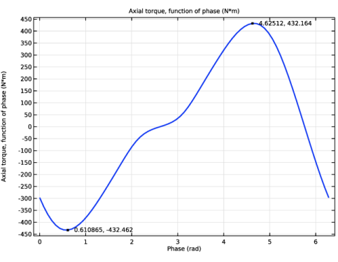
In the Settings window for Global, click Add Expression in the upper-right corner of the y-Axis Data section. From the menu, choose Component 1 (comp1) > Magnetic Machinery, Rotating, Time Periodic > Mechanical > mmtp.drcon1.Tax_tpph - Axial torque, function of phase - N·m.
|
|
3
|
|
4
|
|
5
|
|
6
|
|
1
|
|
2
|
|
3
|
Select the Show x-coordinate checkbox.
|
|
4
|
|
5
|
|
1
|
|
2
|
|
1
|
|
2
|
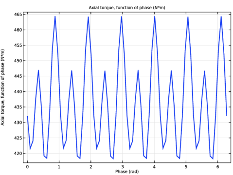
In the Settings window for Global Evaluation, click Add Expression in the upper-right corner of the Expressions section. From the menu, choose Component 1 (comp1) > Magnetic Machinery, Rotating, Time Periodic > Mechanical > mmtp.drcon1.Tax_tpavg - Axial torque, time periodic average - N·m.
|
|
3
|
|
1
|
|
2
|
|
1
|
In the Model Builder window, under Component 1 (comp1) > Magnetic Machinery, Rotating, Time Periodic (mmtp) click Rotating Domain 1.
|
|
2
|
|
3
|
|
1
|
|
2
|
|
3
|
|
4
|
|
1
|
In the Model Builder window, expand the Results > Datasets node, then click Study 1/Solution 1 (sol1).
|
|
2
|
|
3
|
|
1
|
|
2
|
|
1
|
|
2
|
|
1
|
|
2
|
In the Settings window for Global, click Add Expression in the upper-right corner of the y-Axis Data section. From the menu, choose Component 1 (comp1) > Magnetic Machinery, Rotating, Time Periodic > Winding > Voltage > mmtp.wnd1.aPh1.V_tpph - Winding phase voltage, function of phase - V.
|
|
3
|
Locate the y-Axis Data section. In the table, enter the following settings:
|
|
4
|
|
5
|
|
6
|
|
1
|
|
2
|
|
1
|
|
2
|
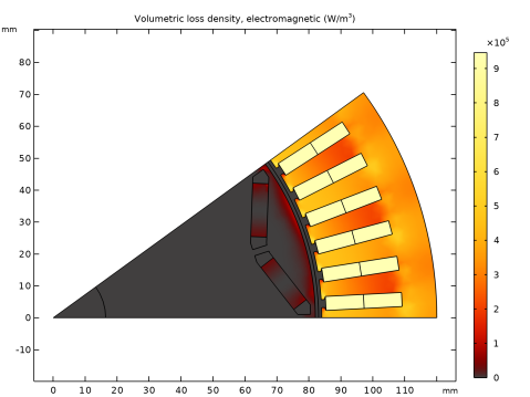
In the Settings window for Surface, click Replace Expression in the upper-right corner of the Expression section. From the menu, choose Component 1 (comp1) > Magnetic Machinery, Rotating, Time Periodic > Heating and losses > mmtp.Qh - Volumetric loss density, electromagnetic - W/m³.
|
|
3
|
|
4
|
|
5
|
|
6
|
|
1
|
In the Model Builder window, under Results > Main Results right-click Global Evaluation 1 and choose Duplicate.
|
|
2
|
|
1
|
|
2
|
|
3
|
|
4
|
Click Add Expression in the upper-right corner of the Expressions section. From the menu, choose Component 1 (comp1) > Magnetic Machinery, Rotating, Time Periodic > Heating and losses > mmtp.Qh - Volumetric loss density, electromagnetic - W/m³.
|
|
5
|
Locate the Expressions section. In the table, enter the following settings:
|
|
1
|
|
2
|
|
3
|
|
4
|
Locate the Expressions section. In the table, enter the following settings:
|
|
1
|
|
2
|
|
3
|
|
4
|
Locate the Expressions section. In the table, enter the following settings:
|
|
1
|
|
2
|
|
3
|
|
4
|
Locate the Expressions section. In the table, enter the following settings:
|
|
1
|
|
2
|
|
3
|
Select the Transpose checkbox.
|
|
4
|
|
5
|
Select the Keep child nodes checkbox.
|
|
6
|
|
7
|
|
8
|
|
1
|
|
2
|
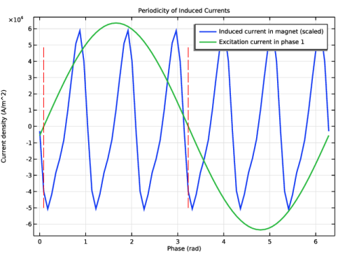
In the Settings window for 1D Plot Group, type Periodicity of Induced Currents in the Label text field.
|
|
3
|
|
4
|
Locate the Plot Settings section.
|
|
5
|
|
1
|
|
2
|
|
3
|
Click
|
|
4
|
|
5
|
Click OK.
|
|
6
|
In the Settings window for Point Graph, click Replace Expression in the upper-right corner of the y-Axis Data section. From the menu, choose Component 1 (comp1) > Magnetic Machinery, Rotating, Time Periodic > Currents and charge > mmtp.JZ_tpph - Current density out of plane, function of phase - A/m².
|
|
7
|
|
8
|
Select the Description checkbox. In the associated text field, type Induced current in magnet (scaled).
|
|
9
|
|
10
|
|
11
|
|
12
|
|
13
|
|
14
|
Clear the Solution checkbox.
|
|
15
|
Select the Description checkbox.
|
|
1
|
|
2
|
|
3
|
Click
|
|
4
|
Click
|
|
5
|
|
6
|
Click OK.
|
|
7
|
|
8
|
|
9
|
|
1
|
|
3
|
Locate the y-Coordinates section. In the table, enter the following settings:
|
|
4
|
|
5
|
|
1
|
|
2
|
|
4
|
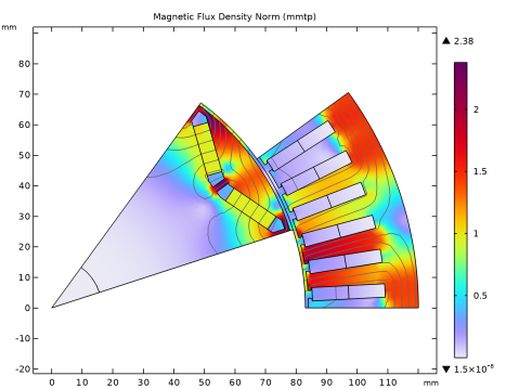
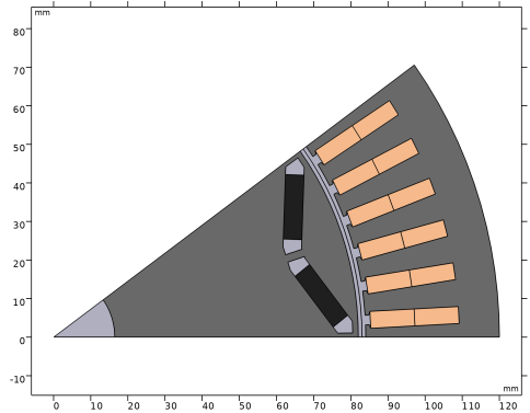
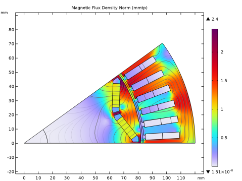 Magnetic flux density distribution at phase angle 0°E.