PDF

Permanent Magnet Motor in 3D
Introduction
Permanent magnet (PM) motors are used in many high end applications, for example in electric and hybrid vehicles. An important design limitation is that the permanent magnets are sensitive to high temperature. The eddy current losses in the steel/iron parts of the motor can easily be reduced by laminating these. However, due to manufacturing limitations, the permanent magnets cannot easily be laminated so the heating can be quite substantial as illustrated in this model.
Model Definition
An 18 pole permanent magnet motor is modeled in 3D. Sector symmetry and axial mirror symmetry is utilized to reduce the computational effort while capturing the full 3D behavior of the device. Figure 1 shows the full PM motor.
Figure 1: Drawing of the permanent magnet motor showing how the rotor and stator iron (gray), stator winding (Cu) and permanent magnets (blue/red depending on radial magnetization) are constructed. The antisymmetric sector is indicated by the dashed line. In addition mirror symmetry in the axial (out-of-plane) direction is utilized.
The conducting part of the rotor is modeled using Ampère’s law:
whereas the nonconducting parts of both the rotor and stator are modeled using a magnetic flux conservation equation for the scalar magnetic potential:
Rotation is modeled using the ready-made physics interface for rotating machinery. The central part of the geometry, containing the rotor and part of the air-gap, is modeled as rotating relative to the coordinate system of the stator. The rotor and the stator are created as two separate geometry objects, so it is required to use an assembly (see the Geometry chapter in the COMSOL Multiphysics Reference Manual for details).
The electromagnetic losses in the magnets are computed with the Time to Frequency Losses study. This can later be used as a distributed, time-averaged, heat source in a separate heat transfer analysis (not included). The thermal time scale is typically much larger than the time variation of the eddy current losses so separating the electromechanical and thermal analyses is usually necessary for computational efficiency.
Results and Discussion
Figure 2 shows the magnetic flux density for the motor in it’s stationary state, that is the initial conditions for the time-dependent simulation. In this state the coil current is zero.
Figure 2: Magnetic flux density from the permanent magnets only with the rotor at rest.
Figure 3 shows the magnetic flux density for the motor after revolving one sector angle. In this plot the air and coil domains are excluded in order to get a better view.
Figure 3: Magnetic flux density after revolving one sector angle.
Figure 4 shows the time evolution of the total eddy current losses in the magnet.
Figure 4: The eddy current loss in the magnets as a function of time.
Figure 5 shows the time averaged eddy current loss power in the magnet in a period.
Figure 5: Time averaged eddy current loss power density in the magnet.
Application Library path: ACDC_Module/Devices,_Motors_and_Generators/pm_motor_3d
Modeling Instructions
From the File menu, choose New.
New
In the New window, click  Model Wizard.
Model Wizard
1
In the Model Wizard window, click  3D.
2
In the Select Physics tree, select AC/DC > Electromagnetics and Mechanics > Rotating Machinery, Magnetic (rmm).
3
Click Add.
4
Click  Study.
5
In the Select Study tree, select General Studies > Stationary.
6
Global Definitions
Parameters 1
1
In the Model Builder window, under Global Definitions click Parameters 1.
2
In the Settings window for Parameters, locate the Parameters section.
3
Click  Load from File.
4
Geometry 1
Import 1 (imp1)
1
In the Geometry toolbar, click  Import.
2
In the Settings window for Import, locate the Source section.
3
Click  Browse.
4
5
Click  Import.
Form Union (fin)
An assembly must be used so that rotor and stator parts can be meshed independently.
1
In the Model Builder window, under Component 1 (comp1) > Geometry 1 click Form Union (fin).
2
In the Settings window for Form Union/Assembly, locate the Form Union/Assembly section.
3
From the Action list, choose Form an assembly.
4
Select the Create imprints checkbox.
5
In the Geometry toolbar, click  Build All.
6
Click the  Wireframe Rendering button in the Graphics toolbar.
Materials
Proceed to define materials.
Add Material
1
In the Materials toolbar, click  Add Material to open the Add Material window.
2
Go to the Add Material window.
3
In the tree, select Built-in > Air.
4
Click the Add to Component button in the window toolbar.
5
In the tree, select AC/DC > Soft Iron (Without Losses).
6
Click the Add to Component button in the window toolbar.
7
In the tree, select AC/DC > Hard Magnetic Materials > Sintered NdFeB Grades (Chinese Standard) > N50 (Sintered NdFeB).
8
Click the Add to Component button in the window toolbar.
9
In the tree, select Built-in > Aluminum.
10
Click the Add to Component button in the window toolbar.
11
In the tree, select Built-in > Structural steel.
12
Click the Add to Component button in the window toolbar.
13
In the tree, select Built-in > Copper.
14
Click the Add to Component button in the window toolbar.
15
In the Materials toolbar, click  Add Material to close the Add Material window.
Materials
Soft Iron (Without Losses) (mat2)
1
For the easiest modeling setup a finite conductivity is added wherever the magnetic vector potential formulation is used.
2
In the Settings window for Material, locate the Material Contents section.
3
Custom the magnetic material of the permanent magnet.
Magnet
1
In the Model Builder window, under Component 1 (comp1) > Materials click N50 (Sintered NdFeB) (mat3).
2
In the Settings window for Material, type Magnet in the Label text field.
3
4
Locate the Material Contents section. In the table, enter the following settings:
Aluminum (mat4)
1
In the Model Builder window, click Aluminum (mat4).
2
Some materials, like this one will not be used in the simulation but could be useful later, for example in a heat transfer simulation.
Structural steel (mat5)
1
In the Model Builder window, click Structural steel (mat5).
2
Copper (mat6)
1
In the Model Builder window, click Copper (mat6).
2
Rotating Machinery, Magnetic (rmm)
Proceed to set up the physics. Limit the electromagnetic simulation to the relevant domains.
1
In the Model Builder window, under Component 1 (comp1) click Rotating Machinery, Magnetic (rmm).
2
Magnetic Flux Conservation - air
1
In the Physics toolbar, click  Domains and choose Magnetic Flux Conservation.
2
In the Settings window for Magnetic Flux Conservation, type Magnetic Flux Conservation - air in the Label text field.
3
Locate the Domain Selection section. Click  Paste Selection.
4
In the Paste Selection dialog, type 5-6, 10-11 in the Selection text field.
5
Magnetic Flux Conservation - iron
1
In the Physics toolbar, click  Domains and choose Magnetic Flux Conservation.
2
In the Settings window for Magnetic Flux Conservation, type Magnetic Flux Conservation - iron in the Label text field.
3
Locate the Domain Selection section. Click  Paste Selection.
4
In the Paste Selection dialog, type 12 in the Selection text field.
5
6
In the Settings window for Magnetic Flux Conservation, locate the Constitutive Relation B-H section.
7
From the Magnetization model list, choose B-H curve.
Laminated Core, Ampère’s Law 1
Add a Laminated Core feature to represent the anisotropic magnetization properties of the stator core without having to resolve the electric steel sheets in detail.
1
In the Physics toolbar, click  Domains and choose Laminated Core, Ampère’s Law.
2
In the Settings window for Laminated Core, Ampère’s Law, locate the Domain Selection section.
3
Click  Paste Selection.
4
In the Paste Selection dialog, type 4 in the Selection text field.
5
6
In the Settings window for Laminated Core, Ampère’s Law, locate the Lamination Model section.
7
From the Lamination model list, choose Direction based.
8
Specify the d vector as
Conducting Magnet 1
Now add a magnet. Leaving the default setting, electrical isolation on all boundaries is assumed. It is possible to change this assumption by changing the constraint for induced currents.
1
In the Physics toolbar, click  Domains and choose Conducting Magnet.
2
Loss Calculation 1
In the Physics toolbar, click  Attributes and choose Loss Calculation.
North 1
1
In the Model Builder window, click North 1.
2
South 1
1
In the Model Builder window, click South 1.
2
Domain Coil 1
1
In the Physics toolbar, click  Domains and choose Domain Coil.
2
3
In the Settings window for Domain Coil, locate the Coil section.
4
From the Conductor model list, choose Homogenized multiturn.
5
In the Icoil text field, type I0*sin(omega*t).
6
Locate the Homogenized Conductor section. In the N text field, type 1.
7
From the Coil wire cross-section area list, choose User defined.
8
Find the High-frequency effective loss subsection. Clear the Include harmonic loss checkbox.
9
In the a text field, type a_coil.
Loss Calculation 1
In the Physics toolbar, click  Attributes and choose Loss Calculation.
Geometry Analysis 1
1
In the Model Builder window, click Geometry Analysis 1.
2
In the Settings window for Geometry Analysis, click to expand the Symmetry Specification section.
3
In the FL text field, type 2.
This accounts for the fact that only one half of the coil is included.
Specify the current direction in the coil.
Input 1
1
In the Model Builder window, expand the Geometry Analysis 1 node, then click Input 1.
2
Zoom out to see the direction arrow.
3
Click the  Zoom Extents button in the Graphics toolbar.
Geometry Analysis 1
In the Model Builder window, click Geometry Analysis 1.
Output 1
1
In the Physics toolbar, click  Attributes and choose Output.
2
Rotating Machinery, Magnetic (rmm)
Domain Coil 1
In the Model Builder window, collapse the Component 1 (comp1) > Rotating Machinery, Magnetic (rmm) > Domain Coil 1 node.
Component 1 (comp1)
Rotating Domain 1
1
In the Physics toolbar, click  Moving Mesh and choose Rotating Domain.
2
3
In the Settings window for Rotating Domain, locate the Rotation section.
4
In the α text field, type omega_rotor*t.
5
Locate the Axis section. Specify the urot vector as
Rotating Machinery, Magnetic (rmm)
Force Calculation 1
1
In the Physics toolbar, click  Domains and choose Force Calculation.
2
Gauge Fixing for A-Field 1
Fix the gauge for the magnetic vector potential.
In the Physics toolbar, click  Domains and choose Gauge Fixing for A-Field.
Periodic Condition 1
Set up the periodicity of the model. Use separate features for the stator and rotor and, for vector and scalar potentials respectively.
1
In the Physics toolbar, click  Boundaries and choose Periodic Condition.
2
3
In the Settings window for Periodic Condition, locate the Periodic Condition section.
4
From the Type of periodicity list, choose Antiperiodicity.
Periodic Condition 2
1
Right-click Periodic Condition 1 and choose Duplicate.
2
In the Settings window for Periodic Condition, locate the Boundary Selection section.
3
Click  Clear Selection.
4
Periodic Condition 3
1
Right-click Periodic Condition 2 and choose Duplicate.
2
In the Settings window for Periodic Condition, locate the Boundary Selection section.
3
Click  Clear Selection.
4
Sector Symmetry 1
Add the pair condition for the rotor-stator interface.
1
In the Physics toolbar, click  Pairs and choose Sector Symmetry.
2
In the Settings window for Sector Symmetry, locate the Pair Selection section.
3
4
In the Add dialog, select Identity Boundary Pair 3 (ap3) in the Pairs list.
5
6
In the Settings window for Sector Symmetry, locate the Sector Settings section.
7
In the nsect text field, type n_sectors.
8
From the Type of periodicity list, choose Antiperiodicity.
Arkkio Torque Calculation 1
Add the torque calculation by means of Arkkio’s method.
In the Physics toolbar, click  Domains and choose Arkkio Torque Calculation.
Definitions
Set up variables and other definitions used to define customized output.
Integration - Magnet
1
In the Definitions toolbar, click  Nonlocal Couplings and choose Integration.
2
In the Settings window for Integration, type Integration - Magnet in the Label text field.
3
In the Operator name text field, type intop1_magnet.
4
Integration - Coil
1
Right-click Integration - Magnet and choose Duplicate.
2
In the Settings window for Integration, type Integration - Coil in the Label text field.
3
In the Operator name text field, type intop2_coil.
4
Locate the Source Selection section. Click  Clear Selection.
5
Global Variable Probe 1 - Torque
Define probes to be plotted while solving.
1
In the Definitions toolbar, click  Probes and choose Global Variable Probe.
2
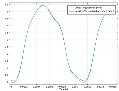
In the Settings window for Global Variable Probe, type Global Variable Probe 1 - Torque in the Label text field.
3
Locate the Expression section. In the Expression text field, type rmm.Tax_1*n_sectors*2.
4
Select the Description checkbox. In the associated text field, type Axial Torque (N*m).
Global Variable Probe 2 - Arkkio’s Torque method
1
Right-click Global Variable Probe 1 - Torque and choose Duplicate.
2
In the Settings window for Global Variable Probe, type Global Variable Probe 2 - Arkkio's Torque method in the Label text field.
3
Locate the Expression section. In the Expression text field, type rmm.Tark_1*2.
4
In the Description text field, type Arkkio's Torque Method (N*m).
Global Variable Probe 3 - Magnet Loss
1
In the Definitions toolbar, click  Probes and choose Global Variable Probe.
2
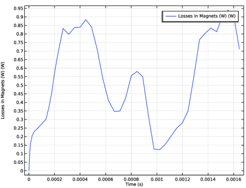
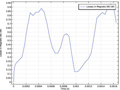
In the Settings window for Global Variable Probe, type Global Variable Probe 3 - Magnet Loss in the Label text field.
3
Locate the Expression section. In the Expression text field, type intop1_magnet(rmm.Qh)*n_sectors*2.
4
Select the Description checkbox. In the associated text field, type Losses in Magnets (W).
5
Click to expand the Table and Window Settings section. From the Plot window list, choose New window.
Global Variable Probe 4 - Coil Loss
1
Right-click Global Variable Probe 3 - Magnet Loss and choose Duplicate.
2
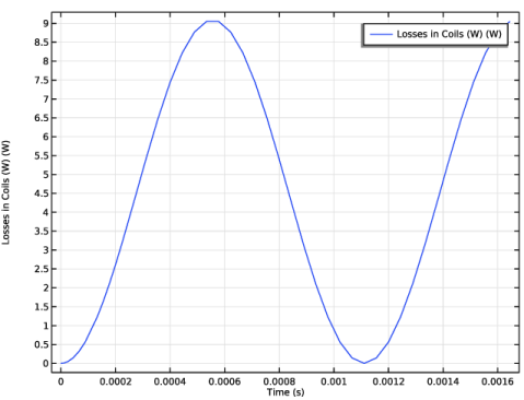
In the Settings window for Global Variable Probe, type Global Variable Probe 4 - Coil Loss in the Label text field.
3
Locate the Expression section. In the Expression text field, type intop2_coil(rmm.Qh)*n_sectors*2.
4
In the Description text field, type Losses in Coils (W).
Definitions
In the Model Builder window, collapse the Component 1 (comp1) > Definitions node.
Rotating Machinery, Magnetic (rmm)
In the Model Builder window, collapse the Component 1 (comp1) > Rotating Machinery, Magnetic (rmm) node.
Mesh 1
Next, create the mesh. Use the mesh suggested by the physics as a starting point.
1
In the Model Builder window, under Component 1 (comp1) click Mesh 1.
2
In the Settings window for Mesh, locate the Physics-Controlled Mesh section.
3
From the Element size list, choose Fine.
4
In the table, clear the Use checkbox for Geometric Analysis, Detail Size.
5
Right-click Component 1 (comp1) > Mesh 1 and choose Edit Physics-Induced Sequence.
Size
In the Model Builder window, under Component 1 (comp1) > Mesh 1 right-click Size and choose Build Selected.
Use a finer mesh on the side of the magnet facing the stator.
Size 1
1
In the Model Builder window, right-click Mesh 1 and choose Size.
2
In the Settings window for Size, locate the Geometric Entity Selection section.
3
From the Geometric entity level list, choose Boundary.
4
5
Locate the Element Size section. Click the Custom button.
6
Locate the Element Size Parameters section.
7
Select the Maximum element size checkbox. In the associated text field, type 0.0005.
8
Click  Build Selected.
The pair boundaries need a finer mesh on the destination boundary so custom meshing is needed for source and destination.
Free Triangular 1
1
In the Mesh toolbar, click  More Generators and choose Free Triangular.
2
Size 1
1
Right-click Free Triangular 1 and choose Size.
2
In the Settings window for Size, locate the Element Size section.
3
Click the Custom button.
4
Locate the Element Size Parameters section.
5
Select the Maximum element size checkbox. In the associated text field, type 0.001.
Free Triangular 2
1
In the Model Builder window, under Component 1 (comp1) > Mesh 1 right-click Free Triangular 1 and choose Duplicate.
2
In the Settings window for Free Triangular, locate the Boundary Selection section.
3
Click  Clear Selection.
4
Size 1
1
In the Model Builder window, expand the Free Triangular 2 node, then click Size 1.
2
In the Settings window for Size, locate the Element Size Parameters section.
3
In the Maximum element size text field, type 0.001/1.25.
4
Click  Build Selected.
5
Click the  Zoom Extents button in the Graphics toolbar.
Free Triangular 3
1
In the Model Builder window, under Component 1 (comp1) > Mesh 1 right-click Free Triangular 2 and choose Duplicate.
2
In the Settings window for Free Triangular, locate the Boundary Selection section.
3
Click  Clear Selection.
4
Size 1
1
In the Model Builder window, expand the Free Triangular 3 node, then click Size 1.
2
In the Settings window for Size, locate the Element Size section.
3
Click the Predefined button.
4
From the Predefined list, choose Extra fine.
5
Click  Build Selected.
The periodic boundaries need identical meshes and this part was set up by the physics.
Identical Mesh 3
1
In the Model Builder window, under Component 1 (comp1) > Mesh 1 right-click Identical Mesh 3 and choose Build Selected.
2
Click the  Zoom Extents button in the Graphics toolbar.
Free Tetrahedral 1
1
In the Model Builder window, click Free Tetrahedral 1.
2
Use the free tetrahedral mesh in all domains except the magnet.
Size 1
1
Right-click Free Tetrahedral 1 and choose Size.
2
In the Settings window for Size, locate the Geometric Entity Selection section.
3
From the Geometric entity level list, choose Edge.
4
5
Locate the Element Size section. Click the Custom button.
6
Locate the Element Size Parameters section.
7
Select the Maximum element size checkbox. In the associated text field, type 0.001/2.
Use a boundary layer mesh to resolve the skin depth in the magnet.
8
Click  Build Selected.
Boundary Layers 1
1
In the Mesh toolbar, click  Boundary Layers.
2
In the Settings window for Boundary Layers, locate the Geometric Entity Selection section.
3
From the Geometric entity level list, choose Domain.
4
Boundary Layer Properties
1
In the Model Builder window, click Boundary Layer Properties.
2
In the Settings window for Boundary Layer Properties, locate the Boundary Selection section.
3
Click  Paste Selection.
4
In the Paste Selection dialog, type 91-92, 94, 99-100, 109-110 in the Selection text field.
5
6
In the Settings window for Boundary Layer Properties, locate the Layers section.
7
In the Number of layers text field, type 5.
8
In the Stretching factor text field, type 1.8.
9
Click  Build Selected.
10
Click the  Go to XY View button in the Graphics toolbar three times.
11
Click the  Zoom Extents button in the Graphics toolbar.
Study 1
Next set up the stationary study that will compute the initial conditions for the time-dependent simulation.
First, solve for the numeric coil.
1
In the Model Builder window, click Study 1.
2
In the Settings window for Study, locate the Study Settings section.
3
Clear the Generate default plots checkbox.
Step 2: Coil Geometry Analysis
1
In the Study toolbar, click  More Study Steps and choose Other > Coil Geometry Analysis.
2
Right-click Step 2: Coil Geometry Analysis and choose Move Up.
3
In the Study toolbar, click  Compute.
Results
Create a custom plot.
Magnetic Flux Density (stationary)
1
In the Results toolbar, click  3D Plot Group.
2
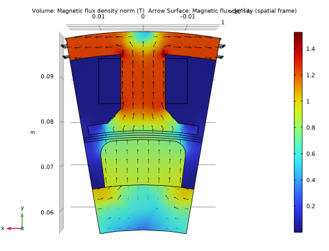
In the Settings window for 3D Plot Group, type Magnetic Flux Density (stationary) in the Label text field.
3
Locate the Plot Settings section. From the Frame list, choose Spatial  (x, y, z).
Volume 1
Right-click Magnetic Flux Density (stationary) and choose Volume.
Arrow Surface 1
1
In the Model Builder window, right-click Magnetic Flux Density (stationary) and choose Arrow Surface.
2
In the Settings window for Arrow Surface, locate the Arrow Positioning section.
3
In the Number of arrows text field, type 2000.
4
Locate the Coloring and Style section. From the Color list, choose Black.
5
In the Magnetic Flux Density (stationary) toolbar, click  Plot.
6
Click the  Zoom Extents button in the Graphics toolbar.
Add Study
Proceed to set up the time-dependent simulation using the stationary solution as initial condition. The latter is necessary as otherwise the permanent magnet would be interpreted as being switched on at t = 0, resulting in an unphysical solution.
1
In the Home toolbar, click  Add Study to open the Add Study window.
2
Go to the Add Study window.
3
Find the Studies subsection. In the Select Study tree, select General Studies > Time Dependent.
4
Click the Add Study button in the window toolbar.
5
In the Home toolbar, click  Add Study to close the Add Study window.
Study 2
1
In the Settings window for Study, locate the Study Settings section.
2
Clear the Generate default plots checkbox.
Step 1: Time Dependent
1
In the Model Builder window, under Study 2 click Step 1: Time Dependent.
2
In the Settings window for Time Dependent, locate the Study Settings section.
3
In the Output times text field, type range(0,time_one_cycle/25,1.5*time_one_cycle).
Proper setup of initial conditions and handling of variables that are not solved for, in this case variables used by the coil geometry analysis, requires some extra attention.
4
Click to expand the Values of Dependent Variables section. Find the Initial values of variables solved for subsection. From the Settings list, choose User controlled.
5
From the Method list, choose Solution.
6
From the Study list, choose Study 1, Stationary.
7
Find the Values of variables not solved for subsection. From the Settings list, choose User controlled.
8
From the Method list, choose Solution.
9
From the Study list, choose Study 1, Stationary.
These steps make sure that you get the desired initial values and use and output the desired values of whatever variables you are not solving for in the current study step.
Solution 3 (sol3)
The setup of the time-dependent solver is almost finished but for models that take some considerable time to simulate, it is good practice to generate some customized graphical output while solving for debugging purposes.
In the Study toolbar, click  Show Default Solver.
Results
Study 2/Solution 3 (sol3)
A dataset for the time-dependent solution was generated with the solver. Use this to create the desired plot to be shown while solving.
First, change the frame to plot in the observer’s frame (spatial).
Current Density, Magnet (transient)
Now, proceed to add the plot.
1
In the Model Builder window, expand the Results > Datasets node.
2
Right-click Results and choose 3D Plot Group.
3
In the Settings window for 3D Plot Group, type Current Density, Magnet (transient) in the Label text field.
4
Locate the Data section. From the Dataset list, choose Study 2/Solution 3 (sol3).
5
Click to expand the Selection section. From the Geometric entity level list, choose Domain.
6
Volume 1
1
Right-click Current Density, Magnet (transient) and choose Volume.
2
In the Settings window for Volume, click Replace Expression in the upper-right corner of the Expression section. From the menu, choose Component 1 (comp1) > Rotating Machinery, Magnetic (Magnetic Fields) > Currents and charge > rmm.normJ - Current density norm - A/m².
Plot the current density magnitude in the magnet only.
Arrow Surface 1
1
In the Model Builder window, right-click Current Density, Magnet (transient) and choose Arrow Surface.
2
In the Settings window for Arrow Surface, click Replace Expression in the upper-right corner of the Expression section. From the menu, choose Component 1 (comp1) > Rotating Machinery, Magnetic (Magnetic Fields) > Currents and charge > rmm.Jx,...,rmm.Jz - Current density (spatial frame).
3
Locate the Arrow Positioning section. In the Number of arrows text field, type 400.
4
Locate the Coloring and Style section. From the Color list, choose Black.
Current Density, Magnet (transient)
Make sure that the geometry outline is following the motion.
1
In the Model Builder window, click Current Density, Magnet (transient).
2
In the Settings window for 3D Plot Group, locate the Plot Settings section.
3
From the Frame list, choose Spatial  (x, y, z).
Study 2
Finally activate the plotting during solution of the newly created plot group.
Step 1: Time Dependent
1
In the Model Builder window, under Study 2 click Step 1: Time Dependent.
2
In the Settings window for Time Dependent, click to expand the Results While Solving section.
3
Select the Plot checkbox.
4
Note that also the probes will be plotted at the internal step rate of the solver which is usually higher than the solution output rate.
Now, it is time to solve the model. This will take of the order of one hour - more or less depending on computer hardware.
5
In the Study toolbar, click  Compute.
Results
Torque
Inspect the probes, start with the torque plot.
Activate legends to distinguish between the curves.
1
In the Model Builder window, under Results click Probe Plot Group 1.
2
In the Settings window for 1D Plot Group, type Torque in the Label text field.
Probe Table Graph 1
1
In the Model Builder window, expand the Torque node, then click Probe Table Graph 1.
2
In the Settings window for Table Graph, click to expand the Legends section.
There is good agreement between Arkkio’s torque and the torque computed using the Maxwell stress tensor.
Next, have a look at the eddy current losses in the magnet.
Losses in Magnets
1
In the Model Builder window, expand the Results > Probe Plot Group 2 node, then click Probe Plot Group 2.
2
In the Settings window for 1D Plot Group, type Losses in Magnets in the Label text field.
Probe Table Graph 1
1
In the Model Builder window, click Probe Table Graph 1.
The magnet losses vary significantly over time.
Finally have a look at the losses in the coil.
Losses in Coils
1
In the Model Builder window, expand the Results > Probe Plot Group 3 node, then click Probe Plot Group 3.
2
In the Settings window for 1D Plot Group, type Losses in Coils in the Label text field.
Probe Table Graph 1
The coil has a prescribed sinusoidal current density giving rise to resistive losses in the copper.
1
In the Model Builder window, click Probe Table Graph 1.
Next, proceed to create custom plots.
Study 2/Solution 3 (5) (sol3)
In the Model Builder window, under Results > Datasets right-click Study 2/Solution 3 (sol3) and choose Duplicate.
Selection
1
In the Results toolbar, click  Attributes and choose Selection.
2
In the Settings window for Selection, locate the Geometric Entity Selection section.
3
From the Geometric entity level list, choose Domain.
4
Datasets with selections can be used as an alternative to adding selections directly on the plot features.
Next, add a plot of the magnetic flux density.
Magnetic Flux Density (transient)
1
In the Results toolbar, click  3D Plot Group.
2
In the Model Builder window, click 3D Plot Group 6.
3
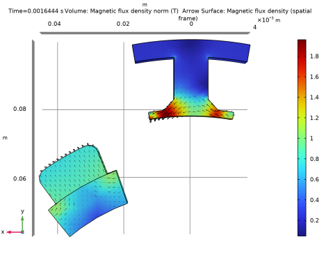
In the Settings window for 3D Plot Group, type Magnetic Flux Density (transient) in the Label text field.
4
Locate the Data section. From the Dataset list, choose Study 2/Solution 3 (5) (sol3).
5
Locate the Plot Settings section. From the Frame list, choose Spatial  (x, y, z).
Volume 1
Right-click Magnetic Flux Density (transient) and choose Volume.
Arrow Surface 1
1
In the Model Builder window, right-click Magnetic Flux Density (transient) and choose Arrow Surface.
2
In the Settings window for Arrow Surface, locate the Arrow Positioning section.
3
In the Number of arrows text field, type 2000.
4
Locate the Coloring and Style section. From the Color list, choose Black.
5
In the Magnetic Flux Density (transient) toolbar, click  Plot.
6
Click the  Zoom Extents button in the Graphics toolbar.
The magnetic flux density in the magnet and iron is shown.
Add Study
1
In the Home toolbar, click  Add Study to open the Add Study window.
2
Go to the Add Study window.
3
Find the Studies subsection. In the Select Study tree, select Preset Studies for Selected Physics Interfaces > Time-to-Frequency Losses.
4
Click the Add Study button in the window toolbar.
5
In the Home toolbar, click  Add Study to close the Add Study window.
Loss Calculation
1
In the Settings window for Study, locate the Study Settings section.
2
Clear the Generate default plots checkbox.
3
In the Label text field, type Loss Calculation.
Step 1: Time-to-Frequency Losses
1
In the Model Builder window, under Loss Calculation click Step 1: Time-to-Frequency Losses.
2
In the Settings window for Time-to-Frequency Losses, locate the Study Settings section.
3
From the Input study list, choose Study 2, Time Dependent.
4
In the Electrical period text field, type time_one_cycle.
5
In the Number of harmonics text field, type 12.
6
In the Study toolbar, click  Compute.
Results
Loss Density in Magnets
1
In the Results toolbar, click  3D Plot Group.
2
In the Settings window for 3D Plot Group, type Loss Density in Magnets in the Label text field.
3
Locate the Data section. From the Dataset list, choose Loss Calculation/Solution 4 (sol4).
Volume 1
1
Right-click Loss Density in Magnets and choose Volume.
2
In the Settings window for Volume, locate the Expression section.
3
In the Expression text field, type rmm.Qh.
Selection 1
1
Right-click Volume 1 and choose Selection.
2
Loss Density in Magnets
1
In the Model Builder window, under Results click Loss Density in Magnets.
2
In the Loss Density in Magnets toolbar, click  Plot.
Volume Integration 1
1
In the Results toolbar, click  More Derived Values and choose Integration > Volume Integration.
2
In the Settings window for Volume Integration, locate the Data section.
3
From the Dataset list, choose Loss Calculation/Solution 4 (sol4).
4
5
Locate the Expressions section. In the table, enter the following settings:
6
Click  Evaluate.
The total loss power of the magnet is about 0.5 W.
Root
Finally add a suitable thumbnail to the model.
1
In the Model Builder window, click the root node.
2
In the root node’s Settings window, locate the Presentation section.
3
Find the Thumbnail subsection. Click Set from Graphics Window.