PDF

Permanent Magnet Motor with Efficiency Map
Introduction
This example demonstrates how to model the interaction between electromagnetic losses and temperature in an electrical motor. Firstly the convergence of electromagnetic losses with temporal resolution is investigated. Secondly a sweep over a range of speeds, torque levels and temperatures is performed in order to create the motor efficiency map. The focus of this tutorial is on the multiphysics coupling and so the electromagnetic and thermal aspects not directly related to this are simplified.
Model Definition
The electromagnetic part of this example is modeled using the Magnetic Machinery Time Periodic interface which directly solves for the steady-state operation. This means it solves for the amount of time in which the electromagnetic field is periodic or repeating itself without resolving any startup transients. With a time periodic solution the space dependent time average electromagnetic losses are easily included in the Heat Transfer interface with the Electromagnetic Heating multiphysics coupling. In return the temperature is used to govern the electric resistance of stator winding and the remanent flux density of rotor magnets, both of which will impact the motor efficiency.
Electromagnetic Considerations
The motor geometry is reduced to the smallest sector which can represent the spatial periodicity of the magnetic field as shown in Figure 1. For most rotating machinery designs the number of sectors corresponding with field periodicity is generally found by Nsec = gcd(NpNs), where Np and Ns are the number of poles, and where gcd() finds the greatest common divisor of these integers.
Figure 1: Modeled motor geometry capturing spatial periodicity of the magnetic field.
The time period for which the magnetic field is repeating itself is for most synchronous machine cases equivalent to the period of electrical excitation. In a synchronous machine the excitation frequency is given by fel = ωrot ⋅ Np/2 where ωrot is the shaft speed, and hence the excitation time period is τel = 1el. This is the time it takes the rotor to rotate an angle spanning exactly one pole pair or two poles.
It is not always however the induced currents have the same time periodicity as the excitation even for a synchronous machine. Isolated the induced currents tend to be periodic with the time it takes the rotor to rotate through an angle of 360°/Nsec, or corresponding with the geometrical periodicity.
This means the periodic time of the induced currents in this model is τind = 1/(ωrot ⋅ Nsec) = 2.5/fel, which unfortunately does not encompass an integer number of excitation periods. The time period at which both the induced currents and the excitation are periodic will in this case correspond to the time taken for a full mechanical revolution τall = 1rot. Solving for a full mechanical revolution can be quite resource demanding in terms of solution time and memory requirements however. Hence a study of the temporal resolution or number of time frames required to achieve good convergence of key results is performed.
The coils are represented as homogenized multiturn conductors which is a fair simplification when the conductor cross section is far smaller than the conductor skin depth. This means all coil conductors are evenly distributed inside a single domain representing the coil cross section. When defining the temperature dependent electric resistivity for such a coil the average temperature of the same domain should be used:
(1).
The temperature dependence of magnet remanent flux density can be expressed similarly:
(2).
Here, Br_ref and Tref represent the reference flux density and temperature, and αBr represents the remanent flux reversible temperature coefficient of the magnet material.
Thermal Considerations
The Electromagnetic Heating multiphysics coupling automatically configures the space dependent electromagnetic loss as a volumetric heat source in the Heat Transfer in Solids interface. This can also be done manually by adding a Heat Source feature and specifying the Electromagnetic Volumetric loss density variable mmtp.Qh as a General source for the relevant domains.
In an electrical motor there are several thermal barriers which contribute significantly to temperature distribution but which are very thin compared to other geometrical details. Typical examples are the insulation around coils and the thermal contact between stator core and motor housing. One way to account for this without resorting to a very detailed mesh is to specify these thermal barriers with the Thin Layer feature.
Figure 2: Thin layer accounts for the thermal barrier around coils and between stator core and motor housing.
The cooling of the motor is in this example simplified to Heat Flux boundary conditions on the outer surface of the motor housing and on internal surfaces adjacent to the airgap between rotor and stator. For the airgap cooling the average temperature of stator solid materials is used as External temperature, or temperature of air in airgap, and a modest heat transfer coefficient of 50 W/(m2·K) is used to represent moderate cooling by forced convection of air on these boundaries.
Results and Discussion
When varying the number of time frames solved for in the Magnetic Machinery Time Periodic interface, it is clear that a coarse temporal resolution overestimates the torque and consequently the shaft power, and underestimates the losses in most components. On the other hand, while solutions with finer temporal resolution converges both in terms of output power and losses, they will require substantial solution time to compute an entire efficiency map. To strike a balance between accuracy and computational cost using 120 time frames seems appropriate in this particular case. The necessary number of frames might be different for other motor designs and is particularly influenced by the time periodicity of the quantities of interest.
Figure 3: Torque and losses as function of number of time frames for one revolution.
In order to generate an efficiency map, the electromagnetic and thermal simulation is run for a range of speeds and current amplitudes spanning the operational space intended for the motor. A plot of electromagnetic loss distribution of the four corner operating points of this space provides an impression of the magnitude of the key loss mechanisms at play.
Figure 4: Electromagnetic loss distribution of four operating points.
It can be seen that the current driven losses are primarily contained in the winding in top left plot of Figure 4. On the other hand the speed driven losses are prominent in both magnets and stator core in bottom right plot of Figure 4. When these two loss mechanisms are combined in top right plot of Figure 4, it is interesting to note a slight asymmetric distribution of losses in magnets and at tip of stator teeth coinciding with the anticlockwise rotational direction.
A similar plot of the temperature distribution provides insight into the effect these losses has on the temperature of the different components.
Figure 5: Temperature distribution of four operating points.
As seen in Figure 5, the temperature of rotor and most importantly magnets is dependent on the stator temperature as it is only cooled by air in the airgap.
The efficiency map is generated by solving for four different speeds and five different current levels giving a total of 20 operating points.
.
Figure 6: Electromagnetic loss distribution of four operating points.
The efficiency in Figure 6, is plotted against torque and speed and shows a slanted top boundary. This shows the effect of diminishing motor torque for the same amount of stator current as the temperature of the magnets elevate with increasing rotor speed.
Application Library path: ACDC_Module/Devices,_Motors_and_Generators/pm_motor_2d_efficiency_map
Modeling Instructions
From the File menu, choose New.
New
In the New window, click  Model Wizard.
Model Wizard
1
In the Model Wizard window, click  2D.
2
Geometry 1
1
In the Model Builder window, under Component 1 (comp1) click Geometry 1.
2
In the Settings window for Geometry, locate the Units section.
3
From the Length unit list, choose mm.
Global Definitions
Parameters 1
1
In the Model Builder window, under Global Definitions click Parameters 1.
2
In the Settings window for Parameters, locate the Parameters section.
3
Click  Load from File.
4
Part Libraries
1
In the Home toolbar, click  Windows and choose Part Libraries.
2
In the Model Builder window, under Component 1 (comp1) click Geometry 1.
3
In the Part Libraries window, select AC/DC Module > Rotating Machinery 2D > Rotors > Internal > surface_mounted_magnet_internal_rotor_2d in the tree.
4
Click  Add to Geometry.
Geometry 1
Internal Rotor – Surface Mounted Magnets 1 (pi1)
1
In the Model Builder window, under Component 1 (comp1) > Geometry 1 click Internal Rotor – Surface Mounted Magnets 1 (pi1).
2
In the Settings window for Part Instance, locate the Input Parameters section.
3
4
Click to expand the Domain Selections section. In the table, select the Keep checkboxes for Shaft, Rotor iron, Rotor Magnets, Rotor solid domains, Rotor air, and All domains.
Part Libraries
1
In the Home toolbar, click  Part Libraries.
2
In the Part Libraries window, select AC/DC Module > Rotating Machinery 2D > Stators > External > slotted_external_stator_2d in the tree.
3
Click  Add to Geometry.
Geometry 1
External Stator – Slotted 1 (pi2)
1
In the Model Builder window, under Component 1 (comp1) > Geometry 1 click External Stator – Slotted 1 (pi2).
2
In the Settings window for Part Instance, locate the Input Parameters section.
3
4
Locate the Domain Selections section. In the table, select the Keep checkboxes for Stator iron and Stator slots.
Form Union (fin)
1
In the Model Builder window, under Component 1 (comp1) > Geometry 1 click Form Union (fin).
2
In the Settings window for Form Union/Assembly, locate the Form Union/Assembly section.
3
From the Action list, choose Form an assembly.
4
In the Home toolbar, click  Build All.
5
Click the  Zoom Extents button in the Graphics toolbar.
Next, create a few selections and operators that will simplify the configuration of the physics.
Definitions
Stator Housing
1
In the Definitions toolbar, click  Explicit.
2
In the Settings window for Explicit, type Stator Housing in the Label text field.
3
Solid Materials
1
In the Definitions toolbar, click  Union.
2
In the Settings window for Union, type Solid Materials in the Label text field.
3
Locate the Input Entities section. Under Selections to add, click  Add.
4
In the Add dialog, in the Selections to add list, choose Stator Housing, Shaft (Internal Rotor – Surface Mounted Magnets 1), Rotor iron (Internal Rotor – Surface Mounted Magnets 1), Rotor Magnets (Internal Rotor – Surface Mounted Magnets 1), Stator iron (External Stator – Slotted 1), and Stator slots (External Stator – Slotted 1).
5
Solid Materials - External Boundaries
1
In the Definitions toolbar, click  Adjacent.
2
In the Settings window for Adjacent, type Solid Materials - External Boundaries in the Label text field.
3
Locate the Input Entities section. Under Input selections, click  Add.
4
In the Add dialog, select Solid Materials in the Input selections list.
5
Airgap Heat Flux Boundaries
1
In the Model Builder window, right-click Selections and choose Disk.
2
In the Settings window for Disk, type Airgap Heat Flux Boundaries in the Label text field.
3
Locate the Geometric Entity Level section. From the Level list, choose Boundary.
4
Locate the Input Entities section. From the Entities list, choose From selections.
5
Under Selections, click  Add.
6
In the Add dialog, select Solid Materials - External Boundaries in the Selections list.
7
8
In the Settings window for Disk, locate the Size and Shape section.
9
In the Outer radius text field, type 18.
10
In the Inner radius text field, type 11.
11
Locate the Output Entities section. From the Include entity if list, choose Entity inside disk.
Laminated Core - Housing Boundaries
1
Right-click Selections and choose Disk.
2
In the Settings window for Disk, type Laminated Core - Housing Boundaries in the Label text field.
3
Locate the Geometric Entity Level section. From the Level list, choose Boundary.
4
Locate the Size and Shape section. In the Outer radius text field, type 25.5.
5
In the Inner radius text field, type 24.5.
6
Locate the Output Entities section. From the Include entity if list, choose Entity inside disk.
Winding Insulation Boundaries
1
In the Definitions toolbar, click  Adjacent.
2
In the Settings window for Adjacent, type Winding Insulation Boundaries in the Label text field.
3
Locate the Input Entities section. Under Input selections, click  Add.
4
In the Add dialog, select Stator slots (External Stator – Slotted 1) in the Input selections list.
5
Water Jacket - External Boundaries
1
Right-click Selections and choose Disk.
2
In the Settings window for Disk, type Water Jacket - External Boundaries in the Label text field.
3
Locate the Geometric Entity Level section. From the Level list, choose Boundary.
4
Locate the Size and Shape section. In the Outer radius text field, type 28.8.
5
In the Inner radius text field, type 27.5.
6
Locate the Output Entities section. From the Include entity if list, choose Entity inside disk.
Stator Solid Materials
1
In the Definitions toolbar, click  Union.
2
In the Settings window for Union, type Stator Solid Materials in the Label text field.
3
Locate the Input Entities section. Under Selections to add, click  Add.
4
In the Add dialog, in the Selections to add list, choose Stator Housing, Stator iron (External Stator – Slotted 1), and Stator slots (External Stator – Slotted 1).
5
Average 1 - Winding
1
In the Definitions toolbar, click  Nonlocal Couplings and choose Average.
2
In the Settings window for Average, type Average 1 - Winding in the Label text field.
3
Locate the Source Selection section. From the Selection list, choose Stator slots (External Stator – Slotted 1).
Average 2 - Stator Solid Materials
1
In the Definitions toolbar, click  Nonlocal Couplings and choose Average.
2
In the Settings window for Average, type Average 2 - Stator Solid Materials in the Label text field.
3
Locate the Source Selection section. From the Selection list, choose Stator Solid Materials.
Add Physics
1
In the Home toolbar, click  Add Physics to open the Add Physics window.
2
Go to the Add Physics window.
3
In the tree, select AC/DC > Electromagnetics and Mechanics > Magnetic Machinery, Rotating, Time Periodic (mmtp).
4
Click the Add to Component 1 button in the window toolbar.
5
In the tree, select Heat Transfer > Heat Transfer in Solids (ht).
6
Click the Add to Component 1 button in the window toolbar.
7
In the Home toolbar, click  Add Physics to close the Add Physics window.
Definitions
In the Model Builder window, collapse the Component 1 (comp1) > Definitions node.
Add Material
1
In the Materials toolbar, click  Add Material to open the Add Material window.
2
Go to the Add Material window.
3
In the tree, select Built-in > Air.
4
Click the Add to Component button in the window toolbar.
5
In the tree, select AC/DC > Soft Iron (Without Losses).
6
Click the Add to Component button in the window toolbar.
7
In the tree, select AC/DC > Copper.
8
Click the Add to Component button in the window toolbar.
9
In the tree, select AC/DC > Hard Magnetic Materials > Sintered NdFeB Grades (Chinese Standard) > N54 (Sintered NdFeB).
10
Click the Add to Component button in the window toolbar.
11
In the tree, select Built-in > High-strength alloy steel.
12
Click the Add to Component button in the window toolbar.
13
In the Materials toolbar, click  Add Material to close the Add Material window.
Materials
Soft Iron (Without Losses) (mat2)
1
2
In the Settings window for Material, locate the Material Contents section.
3
For the coil domains, specify a value for the thermal conductivity representing the in-plane bulk property of insulated copper strands.
Copper (mat3)
1
In the Model Builder window, click Copper (mat3).
2
In the Settings window for Material, locate the Geometric Entity Selection section.
3
From the Selection list, choose Stator slots (External Stator – Slotted 1).
4
Locate the Material Contents section. In the table, enter the following settings:
N54 (Sintered NdFeB) (mat4)
1
In the Model Builder window, click N54 (Sintered NdFeB) (mat4).
2
In the Settings window for Material, locate the Geometric Entity Selection section.
3
From the Selection list, choose Rotor Magnets (Internal Rotor – Surface Mounted Magnets 1).
4
Locate the Material Contents section. In the table, enter the following settings:
High-strength alloy steel (mat5)
1
In the Model Builder window, click High-strength alloy steel (mat5).
2
Materials
1
In the Model Builder window, collapse the Component 1 (comp1) > Materials node.
2
In the Model Builder window, under Component 1 (comp1) click Materials.
3
In the Settings window for Materials, in the Graphics window toolbar, clicknext to  Colors, then choose Show Material Color and Texture.
4
Click the  Zoom Extents button in the Graphics toolbar.
Magnetic Machinery, Rotating, Time Periodic (mmtp)
1
In the Model Builder window, under Component 1 (comp1) click Magnetic Machinery, Rotating, Time Periodic (mmtp).
2
In the Settings window for Magnetic Machinery, Rotating, Time Periodic, locate the Domain Selection section.
3
4
Click  Remove from Selection.
5
6
7
Click  Remove from Selection.
8
9
Locate the Thickness section. In the d text field, type L.
10
Locate the Time Periodic Settings section. In the nTP text field, type Nframes.
11
In the fTP text field, type w_rot.
12
Locate the Motion Settings section. In the npoles text field, type Np.
Rotational Magnetic Continuity 1
In the Physics toolbar, click  Pairs and choose Rotational Magnetic Continuity.
Rotational Periodicity 1
1
In the Physics toolbar, click  Boundaries and choose Rotational Periodicity.
2
Rotating Domain 1
1
In the Physics toolbar, click  Domains and choose Rotating Domain.
2
In the Settings window for Rotating Domain, locate the Rotating Domain section.
3
From the Time periodic rotation list, choose Full mechanical revolution.
Laminated Core 1
1
In the Physics toolbar, click  Domains and choose Laminated Core.
2
Magnet 1
1
In the Physics toolbar, click  Domains and choose Magnet.
2
In the Settings window for Magnet, locate the Domain Selection section.
3
From the Selection list, choose Rotor Magnets (Internal Rotor – Surface Mounted Magnets 1).
4
Locate the Magnet section. From the Pattern type list, choose Circular pattern.
5
From the Type of periodicity list, choose Alternating.
6
Locate the Constitutive Relation B-H section. From the ||  Br   || list, choose User defined. In the associated text field, type PM_Br_ref*(1+PM_alpha*(T-PM_Tref)).
North 1
1
In the Model Builder window, expand the Magnet 1 node, then click North 1.
2
South 1
1
In the Model Builder window, click South 1.
2
Magnetic Machinery, Rotating, Time Periodic (mmtp)
Magnet 1
In the Model Builder window, collapse the Component 1 (comp1) > Magnetic Machinery, Rotating, Time Periodic (mmtp) > Magnet 1 node.
Multiphase Winding 1
1
In the Physics toolbar, click  Domains and choose Multiphase Winding.
2
In the Settings window for Multiphase Winding, locate the Domain Selection section.
3
From the Selection list, choose Stator slots (External Stator – Slotted 1).
4
Locate the Multiphase Winding section. In the Ipk text field, type Ipk.
5
In the αi text field, type init_ang.
6
In the ft text field, type f_el.
7
From the Winding layout configuration list, choose Automatic three phase.
8
In the nslots text field, type Ns.
9
Click Add Phases.
Magnetic Machinery, Rotating, Time Periodic (mmtp)
1
In the Model Builder window, collapse the Component 1 (comp1) > Magnetic Machinery, Rotating, Time Periodic (mmtp) > Multiphase Winding 1 node.
2
In the Model Builder window, click Multiphase Winding 1.
3
In the Settings window for Multiphase Winding, locate the Homogenized Conductor section.
4
In the N text field, type Nturn.
5
In the σ text field, type 1/(Cu_rho0*(1+Cu_alpha*(aveop1(T)-Cu_Tref))).
6
In the f text field, type ff_slot.
Heat Transfer in Solids (ht)
1
In the Model Builder window, under Component 1 (comp1) click Heat Transfer in Solids (ht).
2
In the Settings window for Heat Transfer in Solids, locate the Domain Selection section.
3
From the Selection list, choose Solid Materials.
4
Locate the Physical Model section. In the dz text field, type L.
5
Click to expand the Discretization section. From the Temperature list, choose Linear.
Thin Layer 1 - Laminated Core <> Housing
1
In the Physics toolbar, click  Boundaries and choose Thin Layer.
2
In the Settings window for Thin Layer, type Thin Layer 1 - Laminated Core <> Housing in the Label text field.
3
Locate the Boundary Selection section. From the Selection list, choose Laminated Core - Housing Boundaries.
4
Locate the Shell Properties section. From the Shell type list, choose Nonlayered shell. In the Lth text field, type 0.5e-4[m].
5
Locate the Heat Conduction section. From the k list, choose User defined. In the associated text field, type 0.02.
Thin Layer 2 - Winding Insulation
1
In the Physics toolbar, click  Boundaries and choose Thin Layer.
2
In the Settings window for Thin Layer, type Thin Layer 2 - Winding Insulation in the Label text field.
3
Locate the Boundary Selection section. From the Selection list, choose Winding Insulation Boundaries.
4
Locate the Shell Properties section. From the Shell type list, choose Nonlayered shell. In the Lth text field, type 2e-4[m].
5
Locate the Heat Conduction section. From the k list, choose User defined. In the associated text field, type 0.2.
Heat Flux 1 - Water Jacket
1
In the Physics toolbar, click  Boundaries and choose Heat Flux.
2
In the Settings window for Heat Flux, type Heat Flux 1 - Water Jacket in the Label text field.
3
Locate the Boundary Selection section. From the Selection list, choose Water Jacket - External Boundaries.
4
Locate the Heat Flux section. From the Flux type list, choose Convective heat flux.
5
In the h text field, type 500.
6
In the Text text field, type 25[degC].
Heat Flux 2 - Airgap
1
In the Physics toolbar, click  Boundaries and choose Heat Flux.
2
In the Settings window for Heat Flux, type Heat Flux 2 - Airgap in the Label text field.
3
Locate the Boundary Selection section. From the Selection list, choose Airgap Heat Flux Boundaries.
4
Locate the Heat Flux section. From the Flux type list, choose Convective heat flux.
5
In the h text field, type 50.
6
In the Text text field, type aveop2(T).
Periodic Condition 1
1
In the Physics toolbar, click  Boundaries and choose Periodic Condition.
2
Click the  Select Box button in the Graphics toolbar.
3
Multiphysics
Electromagnetic Heating 1 (emh1)
In the Physics toolbar, click  Multiphysics Couplings and choose Domain > Electromagnetic Heating.
Mesh 1
In the Model Builder window, under Component 1 (comp1) right-click Mesh 1 and choose Edit Physics-Induced Sequence.
Size
1
In the Model Builder window, under Component 1 (comp1) > Mesh 1 click Size.
2
In the Settings window for Size, locate the Element Size section.
3
Click the Custom button.
4
Locate the Element Size Parameters section. In the Curvature factor text field, type 0.6.
5
In the Resolution of narrow regions text field, type 0.5.
Size 1
1
In the Model Builder window, right-click Mesh 1 and choose Size.
2
Drag and drop Size 1 below Size.
3
In the Settings window for Size, locate the Geometric Entity Selection section.
4
From the Geometric entity level list, choose Domain.
5
From the Selection list, choose Stator iron (External Stator – Slotted 1).
6
Click to expand the Element Size Parameters section. Locate the Element Size section. Click the Custom button.
7
Locate the Element Size Parameters section.
8
Select the Maximum element size checkbox. In the associated text field, type 1.
9
Click  Build All.
Mesh 1
In the Model Builder window, collapse the Component 1 (comp1) > Mesh 1 node.
Add Study
1
In the Home toolbar, click  Add Study to open the Add Study window.
2
Go to the Add Study window.
3
Find the Studies subsection. In the Select Study tree, select General Studies > Stationary.
4
Click the Add Study button in the window toolbar.
5
In the Home toolbar, click  Add Study to close the Add Study window.
Study 1 - Convergence with Number of Time Frames
In the Settings window for Study, type Study 1 - Convergence with Number of Time Frames in the Label text field.
Parametric Sweep
1
In the Study toolbar, click  Parametric Sweep.
2
In the Settings window for Parametric Sweep, locate the Study Settings section.
3
4
In order to parameterize the number of time frames solved for it is necessary to disable the Parametric solver.
5
Click to expand the Advanced Settings section. From the Use parametric solver list, choose Off.
6
Select the Reuse solution from previous step checkbox.
Solution 1 (sol1)
While the Heat transfer is heavily influenced by the Magnetic Machinery in this case, the dependence on the coil resistivity and magnetic remanence flux density is only loosely coupled with temperature. For this problem, a Segregated solver is more efficient than the default Fully coupled.
1
In the Study toolbar, click  Show Default Solver.
2
In the Model Builder window, expand the Solution 1 (sol1) node.
3
Right-click Study 1 - Convergence with Number of Time Frames > Solver Configurations > Solution 1 (sol1) > Stationary Solver 1 and choose Segregated.
4
In the Model Builder window, expand the Study 1 - Convergence with Number of Time Frames > Solver Configurations > Solution 1 (sol1) > Stationary Solver 1 > Segregated 1 node, then click Segregated Step.
5
In the Settings window for Segregated Step, type Magnetic Field in the Label text field.
6
Locate the General section. In the Variables list, choose External Temperature (comp1.ht.TextFace) and Temperature (comp1.T).
7
Under Variables, click  Delete.
8
Click to expand the Method and Termination section. From the Termination technique list, choose Tolerance.
9
In the Model Builder window, under Study 1 - Convergence with Number of Time Frames > Solver Configurations > Solution 1 (sol1) > Stationary Solver 1 right-click Segregated 1 and choose Segregated Step.
10
In the Settings window for Segregated Step, type Temperature Field in the Label text field.
11
Locate the General section. Under Variables, click  Add.
12
In the Add dialog, in the Variables list, choose External Temperature (comp1.ht.TextFace) and Temperature (comp1.T).
13
Study 1 - Convergence with Number of Time Frames
Solver Configurations
1
In the Model Builder window, collapse the Study 1 - Convergence with Number of Time Frames > Solver Configurations node.
2
In the Study toolbar, click  Compute.
The following steps will create an Evaluation group and a plot to inspect the convergence with number of time frames.
Results
Evaluation Group 1
In the Results toolbar, click  Evaluation Group.
Global Evaluation 1
1
Right-click Evaluation Group 1 and choose Global Evaluation.
2
In the Settings window for Global Evaluation, click Replace Expression in the upper-right corner of the Expressions section. From the menu, choose Component 1 (comp1) > Magnetic Machinery, Rotating, Time Periodic > Mechanical > mmtp.rcon1.Tax_tpavg - Axial torque, time periodic average - N·m.
3
Locate the Expressions section. In the table, enter the following settings:
Surface Integration 1
1
In the Model Builder window, right-click Evaluation Group 1 and choose Integration > Surface Integration.
2
In the Settings window for Surface Integration, locate the Selection section.
3
From the Selection list, choose Stator slots (External Stator – Slotted 1).
4
Locate the Expressions section. In the table, enter the following settings:
Surface Integration 2
1
Right-click Surface Integration 1 and choose Duplicate.
2
In the Settings window for Surface Integration, locate the Selection section.
3
From the Selection list, choose Stator iron (External Stator – Slotted 1).
4
Locate the Expressions section. In the table, enter the following settings:
Surface Integration 3
1
Right-click Surface Integration 2 and choose Duplicate.
2
In the Settings window for Surface Integration, locate the Selection section.
3
From the Selection list, choose Rotor Magnets (Internal Rotor – Surface Mounted Magnets 1).
4
Locate the Expressions section. In the table, enter the following settings:
Surface Integration 4
1
Right-click Surface Integration 3 and choose Duplicate.
2
In the Settings window for Surface Integration, locate the Selection section.
3
From the Selection list, choose Rotor iron (Internal Rotor – Surface Mounted Magnets 1).
4
Locate the Expressions section. In the table, enter the following settings:
Evaluation Group 1
1
In the Model Builder window, click Evaluation Group 1.
2
In the Settings window for Evaluation Group, locate the Data section.
3
From the Dataset list, choose Study 1 - Convergence with Number of Time Frames/Parametric Solutions 1 (sol2).
4
In the Evaluation Group 1 toolbar, click  Evaluate.
Convergence with Number of Frames
1
In the Results toolbar, click  1D Plot Group.
2
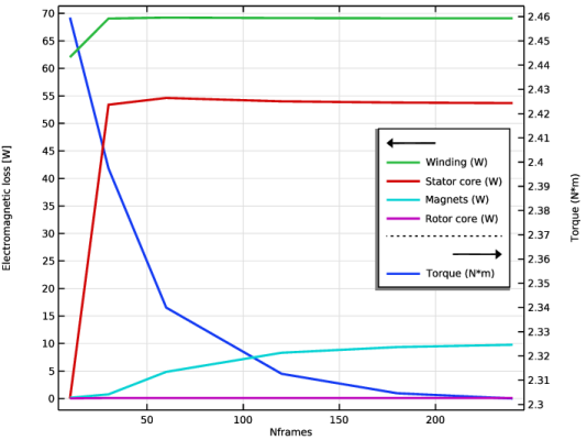
In the Settings window for 1D Plot Group, type Convergence with Number of Frames in the Label text field.
3
Locate the Plot Settings section.
4
Select the y-axis label checkbox. In the associated text field, type Electromagnetic loss [W].
5
Select the Two y-axes checkbox.
6
Locate the Legend section. From the Position list, choose Middle right.
Table Graph 1
1
Right-click Convergence with Number of Frames and choose Table Graph.
2
In the Settings window for Table Graph, locate the Data section.
3
From the Source list, choose Evaluation group.
4
From the x-axis data list, choose Nframes.
5
From the Plot columns list, choose Manual.
6
In the Columns list box, select Torque (N*m).
7
Locate the y-Axis section. Select the Plot on secondary y-axis checkbox.
8
Locate the Coloring and Style section. From the Width list, choose 2.
9
Click to expand the Legends section. Select the Show legends checkbox.
Table Graph 2
1
Right-click Table Graph 1 and choose Duplicate.
2
In the Settings window for Table Graph, locate the Data section.
3
In the Columns list, choose Winding (W), Stator core (W), Magnets (W), and Rotor core (W).
4
Locate the y-Axis section. Clear the Plot on secondary y-axis checkbox.
5
In the Convergence with Number of Frames toolbar, click  Plot.
Results
Convergence with Number of Frames
In the Model Builder window, collapse the Results > Convergence with Number of Frames node.
Update the number of frames and create a new study sweeping over a range of speeds and current levels needed to generate the efficiency map.
Global Definitions
Parameters 1
1
In the Model Builder window, under Global Definitions click Parameters 1.
2
In the Settings window for Parameters, locate the Parameters section.
3
Add Study
1
In the Home toolbar, click  Add Study to open the Add Study window.
2
Go to the Add Study window.
3
Find the Studies subsection. In the Select Study tree, select General Studies > Stationary.
4
Click the Add Study button in the window toolbar.
5
In the Home toolbar, click  Add Study to close the Add Study window.
Study 2 - Efficiency Map
In the Settings window for Study, type Study 2 - Efficiency Map in the Label text field.
Parametric Sweep
1
In the Study toolbar, click  Parametric Sweep.
2
In the Settings window for Parametric Sweep, locate the Study Settings section.
3
From the Sweep type list, choose All combinations.
4
5
6
7
8
Locate the Advanced Settings section. Select the Reuse solution from previous step checkbox.
Solution 9 (sol9)
1
In the Study toolbar, click  Show Default Solver.
2
In the Model Builder window, expand the Solution 9 (sol9) node.
3
In the Model Builder window, expand the Study 2 - Efficiency Map > Solver Configurations > Solution 9 (sol9) > Stationary Solver 1 node.
4
Right-click Study 2 - Efficiency Map > Solver Configurations > Solution 9 (sol9) > Stationary Solver 1 and choose Segregated.
5
In the Model Builder window, expand the Study 2 - Efficiency Map > Solver Configurations > Solution 9 (sol9) > Stationary Solver 1 > Segregated 1 node, then click Segregated Step.
6
In the Settings window for Segregated Step, type Magnetic Field in the Label text field.
7
Locate the General section. In the Variables list, choose External Temperature (comp1.ht.TextFace) and Temperature (comp1.T).
8
Under Variables, click  Delete.
9
Locate the Method and Termination section. From the Termination technique list, choose Tolerance.
10
In the Model Builder window, under Study 2 - Efficiency Map > Solver Configurations > Solution 9 (sol9) > Stationary Solver 1 right-click Segregated 1 and choose Segregated Step.
11
In the Settings window for Segregated Step, type Temperature Field in the Label text field.
12
Locate the General section. Under Variables, click  Add.
13
In the Add dialog, in the Variables list, choose External Temperature (comp1.ht.TextFace) and Temperature (comp1.T).
14
Study 2 - Efficiency Map
Solver Configurations
1
In the Model Builder window, collapse the Study 2 - Efficiency Map > Solver Configurations node.
2
In the Study toolbar, click  Compute.
The following steps duplicate and modify the already existing evaluation group and use it to generate the efficiency map.
Results
Evaluation Group 2
1
In the Model Builder window, under Results right-click Evaluation Group 1 and choose Duplicate.
2
In the Settings window for Evaluation Group, locate the Data section.
3
From the Dataset list, choose Study 2 - Efficiency Map/Solution 9 (sol9).
Global Evaluation 2
1
In the Model Builder window, expand the Evaluation Group 2 node.
2
Right-click Results > Evaluation Group 2 > Global Evaluation 1 and choose Duplicate.
3
In the Settings window for Global Evaluation, locate the Expressions section.
4
Evaluation Group 2
1
In the Model Builder window, click Evaluation Group 2.
2
In the Settings window for Evaluation Group, locate the Transformation section.
3
From the Transformation type list, choose General.
4
Select the Keep child nodes checkbox.
5
In the Expression text field, type gev2/(gev2+int1+int2+int3+int4).
6
In the Column header text field, type Efficiency.
7
In the Evaluation Group 2 toolbar, click  Evaluate.
Evaluation Group 2
1
Go to the Evaluation Group 2 window.
2
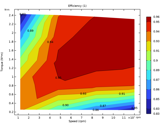
Click the Table Contour button in the window toolbar.
Results
Table Contour 1
1
In the Settings window for Table Contour, locate the Data section.
2
From the y-axis column list, choose Torque (N*m).
Table Contour 2
1
Right-click Results > 2D Plot Group 6 > Table Contour 1 and choose Duplicate.
2
In the Settings window for Table Contour, locate the Coloring and Style section.
3
From the Contour type list, choose Line.
4
Select the Level labels checkbox.
5
In the Precision text field, type 2.
6
From the Label color list, choose Black.
7
From the Color table list, choose RainbowDark.
8
Clear the Color legend checkbox.
9
Click to expand the Title section. From the Title type list, choose None.
Motor Efficiency Map
1
In the Model Builder window, under Results click 2D Plot Group 6.
2
In the Settings window for 2D Plot Group, type Motor Efficiency Map in the Label text field.
3
Locate the Plot Settings section.
4
Select the x-axis label checkbox. In the associated text field, type Speed (rpm).
5
In the Motor Efficiency Map toolbar, click  Plot.
Evaluation Group 2
In the Model Builder window, collapse the Results > Evaluation Group 2 node.
Motor Efficiency Map
In the Model Builder window, collapse the Results > Motor Efficiency Map node.
The remaining steps are rather repetitive and only needed if you want to reproduce Figure 4 and Figure 5 in the Results and Discussion section.
Surface 1
1
In the Model Builder window, expand the Results > Temperature (ht) 1 node, then click Surface 1.
2
In the Settings window for Surface, locate the Data section.
3
From the Dataset list, choose Study 2 - Efficiency Map/Solution 9 (sol9).
4
From the Solution parameters list, choose Manual.
5
From the Parameter value (w_rot (rpm)) list, choose 1200.
6
From the Parameter value (Ipk (A)) list, choose 3.
7
Locate the Expression section. In the Unit field, type degC.
8
Click to expand the Title section. From the Title type list, choose None.
Annotation 1
1
In the Model Builder window, right-click Temperature (ht) 1 and choose Annotation.
2
In the Settings window for Annotation, locate the Data section.
3
From the Dataset list, choose Study 2 - Efficiency Map/Solution 9 (sol9).
4
From the Parameter value (w_rot (rpm)) list, choose 1200.
5
From the Parameter value (Ipk (A)) list, choose 3.
6
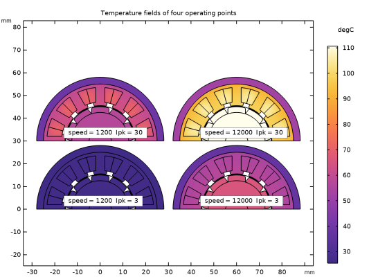
Locate the Annotation section. In the Text text field, type speed = eval(w_rot,rpm,5) Ipk = eval(Ipk,A,3).
7
Locate the Position section. In the X text field, type -16.
8
In the Y text field, type 6.
9
Locate the Coloring and Style section. Clear the Show point checkbox.
10
From the Background color list, choose From theme.
11
Select the Show frame checkbox.
Annotation 1, Surface 1
1
In the Model Builder window, under Results > Temperature (ht) 1, Ctrl-click to select Surface 1 and Annotation 1.
2
Surface 2
1
In the Settings window for Surface, locate the Data section.
2
From the Parameter value (Ipk (A)) list, choose 30.
3
Click to expand the Inherit Style section. From the Plot list, choose Surface 1.
Transformation 1
1
Right-click Surface 2 and choose Transformation.
2
In the Settings window for Transformation, locate the Transformation section.
3
In the Y text field, type 30.
Transformation 1
1
In the Model Builder window, right-click Annotation 2 and choose Transformation.
2
In the Settings window for Transformation, locate the Transformation section.
3
In the Y text field, type 30.
Annotation 2
1
In the Model Builder window, click Annotation 2.
2
In the Settings window for Annotation, locate the Data section.
3
From the Parameter value (Ipk (A)) list, choose 30.
Annotation 2, Surface 2
1
In the Model Builder window, under Results > Temperature (ht) 1, Ctrl-click to select Surface 2 and Annotation 2.
2
Surface 3
1
In the Settings window for Surface, locate the Data section.
2
From the Parameter value (w_rot (rpm)) list, choose 12000.
Transformation 1
1
In the Model Builder window, expand the Surface 3 node, then click Transformation 1.
2
In the Settings window for Transformation, locate the Transformation section.
3
In the X text field, type 60.
Annotation 3
1
In the Model Builder window, under Results > Temperature (ht) 1 click Annotation 3.
2
In the Settings window for Annotation, locate the Data section.
3
From the Parameter value (w_rot (rpm)) list, choose 12000.
Transformation 1
1
In the Model Builder window, expand the Annotation 3 node, then click Transformation 1.
2
In the Settings window for Transformation, locate the Transformation section.
3
In the X text field, type 60.
Annotation 3, Surface 3
1
In the Model Builder window, under Results > Temperature (ht) 1, Ctrl-click to select Surface 3 and Annotation 3.
2
Surface 4
1
In the Settings window for Surface, locate the Data section.
2
From the Parameter value (Ipk (A)) list, choose 3.
Transformation 1
1
In the Model Builder window, expand the Surface 4 node, then click Transformation 1.
2
In the Settings window for Transformation, locate the Transformation section.
3
In the Y text field, type 0.
Annotation 4
1
In the Model Builder window, under Results > Temperature (ht) 1 click Annotation 4.
2
In the Settings window for Annotation, locate the Data section.
3
From the Parameter value (Ipk (A)) list, choose 3.
Transformation 1
1
In the Model Builder window, expand the Annotation 4 node, then click Transformation 1.
2
In the Settings window for Transformation, locate the Transformation section.
3
In the Y text field, type 0.
4
Click the  Zoom Extents button in the Graphics toolbar.
Results
Temperature (ht) 1
1
In the Model Builder window, collapse the Results > Temperature (ht) 1 node.
2
In the Model Builder window, click Temperature (ht) 1.
3
In the Settings window for 2D Plot Group, click to expand the Title section.
4
From the Title type list, choose Manual.
5
In the Title text area, type Temperature fields of four operating points.
6
Clear the Parameter indicator text field.
7
Locate the Color Legend section. Select the Show units checkbox.
8
In the Temperature (ht) 1 toolbar, click  Plot.
Electromagnetic Loss
1
Right-click Temperature (ht) 1 and choose Duplicate.
2
In the Settings window for 2D Plot Group, type Electromagnetic Loss in the Label text field.
3
Locate the Title section. In the Title text area, type Electromagnetic loss distribution of four operating points.
Surface 1
1
In the Model Builder window, expand the Electromagnetic Loss node, then click Surface 1.
2
In the Settings window for Surface, click Replace Expression in the upper-right corner of the Expression section. From the menu, choose Component 1 (comp1) > Magnetic Machinery, Rotating, Time Periodic > Heating and losses > mmtp.Qh - Volumetric loss density, electromagnetic - W/m³.
3
Locate the Coloring and Style section. From the Color table list, choose Rainbow.
Surface 2
1
In the Model Builder window, click Surface 2.
2
In the Settings window for Surface, click Replace Expression in the upper-right corner of the Expression section. From the menu, choose mmtp.Qh - Volumetric loss density, electromagnetic - W/m³.
Surface 3
1
In the Model Builder window, click Surface 3.
2
In the Settings window for Surface, click Replace Expression in the upper-right corner of the Expression section. From the menu, choose mmtp.Qh - Volumetric loss density, electromagnetic - W/m³.
Surface 4
1
In the Model Builder window, click Surface 4.
2
In the Settings window for Surface, click Replace Expression in the upper-right corner of the Expression section. From the menu, choose mmtp.Qh - Volumetric loss density, electromagnetic - W/m³.
Electromagnetic Loss
In the Model Builder window, collapse the Results > Electromagnetic Loss node.