|
|
|
|
1
|
|
2
|
|
3
|
Click Add.
|
|
4
|
In the Select Physics tree, select Acoustics > Pressure Acoustics > Pressure Acoustics, Frequency Domain (acpr).
|
|
5
|
Click Add.
|
|
6
|
In the Select Physics tree, select AC/DC > Electromagnetics and Mechanics > Magnetic Machinery, Rotating, Time Periodic (mmtp).
|
|
7
|
Click Add.
|
|
8
|
Click
|
|
1
|
|
2
|
|
3
|
|
4
|
|
5
|
Browse to the model’s Application Libraries folder and double-click the file pm_motor_2d_campbell_diagram_geom_sequence.mph.
|
|
6
|
|
7
|
|
1
|
|
2
|
|
1
|
|
3
|
|
4
|
|
1
|
In the Model Builder window, under Component 1 (comp1) right-click Definitions and choose Selections > Disk.
|
|
2
|
|
3
|
|
4
|
|
5
|
|
1
|
|
2
|
|
3
|
|
4
|
|
5
|
Click OK.
|
|
1
|
|
2
|
|
3
|
|
4
|
|
5
|
|
6
|
|
7
|
Click OK.
|
|
8
|
|
9
|
|
1
|
|
2
|
Go to the Add Material window.
|
|
3
|
|
4
|
Click the Add to Component button in the window toolbar.
|
|
5
|
|
6
|
Click the Add to Component button in the window toolbar.
|
|
7
|
|
8
|
Click the Add to Component button in the window toolbar.
|
|
9
|
In the tree, select AC/DC > Hard Magnetic Materials > Sintered NdFeB Grades (Chinese Standard) > N42 (Sintered NdFeB).
|
|
10
|
Click the Add to Component button in the window toolbar.
|
|
11
|
|
1
|
|
2
|
Click
|
|
3
|
|
4
|
Click OK.
|
|
1
|
|
3
|
|
1
|
|
2
|
|
3
|
|
4
|
Locate the Material Contents section. In the table, enter the following settings:
|
|
5
|
|
6
|
|
1
|
|
2
|
|
3
|
|
4
|
|
1
|
|
1
|
In the Model Builder window, under Component 1 (comp1) click Pressure Acoustics, Frequency Domain (acpr).
|
|
2
|
In the Settings window for Pressure Acoustics, Frequency Domain, locate the Domain Selection section.
|
|
3
|
|
1
|
|
3
|
In the Settings window for Exterior Field Calculation, locate the Exterior Field Calculation section.
|
|
4
|
|
5
|
|
1
|
In the Model Builder window, under Component 1 (comp1) click Magnetic Machinery, Rotating, Time Periodic (mmtp).
|
|
2
|
In the Settings window for Magnetic Machinery, Rotating, Time Periodic, locate the Domain Selection section.
|
|
3
|
|
4
|
|
5
|
|
6
|
|
7
|
|
1
|
|
1
|
|
1
|
|
2
|
|
3
|
|
4
|
|
5
|
|
1
|
|
1
|
|
1
|
|
2
|
|
3
|
|
4
|
|
5
|
|
6
|
|
7
|
|
8
|
Click Add Phases.
|
|
1
|
|
1
|
|
2
|
Go to the Add Multiphysics window.
|
|
3
|
In the tree, select No Predefined Multiphysics Available for the Selected Physics Interfaces.
|
|
4
|
Find the Select the physics interfaces you want to couple subsection. In the table, clear the Couple checkbox for Magnetic Machinery, Rotating, Time Periodic (mmtp).
|
|
5
|
In the tree, select Acoustics > Acoustic–Structure Interaction > Acoustic–Solid Interaction, Frequency Domain.
|
|
6
|
Click the Add to Component button in the window toolbar.
|
|
7
|
|
1
|
|
2
|
|
3
|
|
1
|
|
2
|
|
3
|
Click the Custom button.
|
|
4
|
|
5
|
|
6
|
|
1
|
|
2
|
|
3
|
|
4
|
|
6
|
|
7
|
Locate the Element Size Parameters section.
|
|
8
|
|
1
|
|
2
|
|
3
|
Click
|
|
4
|
|
5
|
Click OK.
|
|
6
|
|
1
|
|
2
|
|
3
|
|
5
|
|
1
|
|
2
|
|
3
|
|
4
|
|
5
|
|
1
|
|
3
|
|
4
|
|
5
|
|
1
|
|
2
|
|
3
|
|
1
|
|
3
|
|
4
|
|
5
|
Click
|
|
1
|
|
2
|
Go to the Add Study window.
|
|
3
|
Find the Studies subsection. In the Select Study tree, select Preset Studies for Some Physics Interfaces > Eigenfrequency.
|
|
4
|
Click the Add Study button in the window toolbar.
|
|
5
|
|
6
|
Click the Add Study button in the window toolbar.
|
|
7
|
|
8
|
Click the Add Study button in the window toolbar.
|
|
9
|
|
1
|
|
2
|
|
3
|
|
4
|
Clear the Search for eigenfrequencies around shift checkbox.
|
|
5
|
Locate the Physics and Variables Selection section. In the Solve for column of the table, under Component 1 (comp1), clear the checkbox for Pressure Acoustics, Frequency Domain (acpr).
|
|
6
|
In the Solve for column of the table, under Component 1 (comp1) > Multiphysics, clear the checkbox for Acoustic–Structure Boundary 1 (asb1).
|
|
7
|
|
1
|
|
2
|
|
1
|
|
2
|
|
1
|
|
2
|
|
3
|
In the Solve for column of the table, under Component 1 (comp1), clear the checkbox for Solid Mechanics (solid).
|
|
4
|
|
1
|
|
2
|
|
3
|
|
4
|
|
1
|
|
2
|
|
1
|
|
2
|
|
3
|
In the Solve for column of the table, under Component 1 (comp1), clear the checkbox for Magnetic Machinery, Rotating, Time Periodic (mmtp).
|
|
4
|
Click to expand the Values of Dependent Variables section. Find the Values of variables not solved for subsection. From the Settings list, choose User controlled.
|
|
5
|
|
6
|
|
1
|
|
2
|
|
3
|
Click
|
|
5
|
Click to expand the Advanced Settings section. Select the Reuse solution from previous step checkbox.
|
|
1
|
|
2
|
|
3
|
|
4
|
|
1
|
|
2
|
|
1
|
|
2
|
|
4
|
Click Add Expression in the upper-right corner of the y-Coordinates section. From the menu, choose Component 1 (comp1) > Solid Mechanics > Global > solid.freq - Frequency - Hz.
|
|
5
|
Click Add Expression in the upper-right corner of the y-Coordinates section. From the menu, choose solid.freq - Frequency - Hz.
|
|
6
|
|
7
|
|
8
|
|
1
|
|
2
|
|
3
|
|
4
|
Click Add Expression in the upper-right corner of the y-Axis Data section. From the menu, choose Component 1 (comp1) > Solid Mechanics > Global > solid.freq - Frequency - Hz.
|
|
5
|
|
6
|
|
7
|
|
1
|
|
2
|
|
3
|
|
4
|
|
1
|
|
2
|
|
3
|
|
4
|
|
5
|
Select the Show units checkbox.
|
|
6
|
|
1
|
|
2
|
|
3
|
|
4
|
|
5
|
|
1
|
|
2
|
|
3
|
|
4
|
|
5
|
|
6
|
|
7
|
|
1
|
In the Model Builder window, expand the Exterior-Field Sound Pressure Level (acpr) node, then click Radiation Pattern 1.
|
|
2
|
|
3
|
|
4
|
|
5
|
|
6
|
|
7
|
|
8
|
|
1
|
|
2
|
|
3
|
|
4
|
|
5
|
|
6
|
|
7
|
|
1
|
In the Model Builder window, expand the Exterior-Field Pressure (acpr) node, then click Radiation Pattern 1.
|
|
2
|
|
3
|
|
4
|
|
5
|
|
6
|
|
7
|
|
8
|
|
1
|
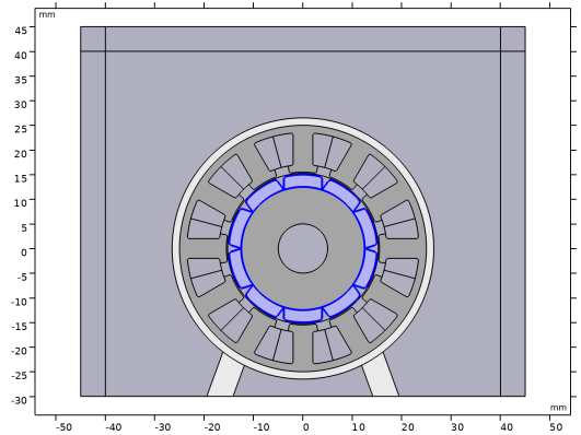
In the Model Builder window, expand the Magnetic Flux Density Norm (mmtp) node, then click Surface 1.
|
|
2
|
In the Settings window for Surface, click Replace Expression in the upper-right corner of the Expression section. From the menu, choose Component 1 (comp1) > Magnetic Machinery, Rotating, Time Periodic > Magnetic > mmtp.normB_tpph - Magnetic flux density norm, function of phase - T.
|
|
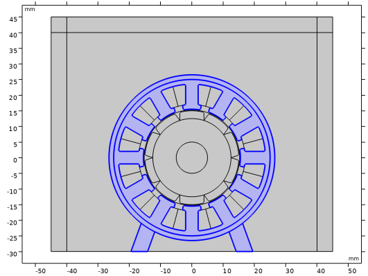
1
|
|
2
|
In the Settings window for Contour, click Replace Expression in the upper-right corner of the Expression section. From the menu, choose Component 1 (comp1) > Magnetic Machinery, Rotating, Time Periodic > Magnetic > mmtp.AZ_tpph - Magnetic vector potential out of plane, function of phase - Wb/m.
|
|
1
|
|
2
|
|
3
|
|
4
|
|
5
|
|
6
|
|
7
|
|
8
|
|
1
|
|
2
|
|
3
|
Locate the Data section. From the Dataset list, choose Study 2 - Electromagnetic Forces/Solution 2 (sol2).
|
|
4
|
|
1
|
|
2
|
|
3
|
|
4
|
|
5
|
|
6
|
|
1
|
|
2
|
|
3
|
|
1
|
|
2
|
|
3
|
|
4
|
|
5
|
|
6
|
|
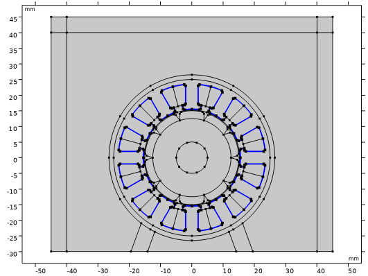
1
|
In the Model Builder window, under Results > Magnetic force harmonics, Ctrl-click to select Line 1 and Arrow Line 1.
|
|
2
|
Right-click and choose Duplicate.
|
|
1
|
|
2
|
|
3
|
|
1
|
|
2
|
|
3
|
|
4
|
|
5
|
|
1
|
|
2
|
|
3
|
|
1
|
In the Model Builder window, under Results > Magnetic force harmonics, Ctrl-click to select Line 2 and Arrow Line 2.
|
|
2
|
Right-click and choose Duplicate.
|
|
1
|
In the Model Builder window, expand the Results > Magnetic force harmonics > Line 3 node, then click Transformation 1.
|
|
2
|
|
3
|
|
1
|
|
2
|
|
3
|
|
4
|
|
1
|
|
2
|
|
3
|
|
1
|
In the Model Builder window, under Results > Magnetic force harmonics, Ctrl-click to select Line 3 and Arrow Line 3.
|
|
2
|
Right-click and choose Duplicate.
|
|
1
|
In the Model Builder window, expand the Results > Magnetic force harmonics > Line 4 node, then click Transformation 1.
|
|
2
|
|
3
|
|
1
|
|
2
|
|
3
|
|
4
|
|
1
|
|
2
|
|
3
|
|
1
|
In the Model Builder window, under Results > Magnetic force harmonics, Ctrl-click to select Line 4 and Arrow Line 4.
|
|
2
|
Right-click and choose Duplicate.
|
|
1
|
In the Model Builder window, expand the Results > Magnetic force harmonics > Line 5 node, then click Transformation 1.
|
|
2
|
|
3
|
|
4
|
|
1
|
|
2
|
|
3
|
|
4
|
|
5
|
|
1
|
|
2
|
|
3
|
|
4
|
|
1
|
In the Model Builder window, under Results > Magnetic force harmonics, Ctrl-click to select Line 5 and Arrow Line 5.
|
|
2
|
Right-click and choose Duplicate.
|
|
1
|
In the Model Builder window, expand the Results > Magnetic force harmonics > Line 6 node, then click Transformation 1.
|
|
2
|
|
3
|
|
1
|
|
2
|
|
3
|
|
4
|
|
1
|
|
2
|
|
3
|
|
1
|
In the Model Builder window, under Results > Magnetic force harmonics, Ctrl-click to select Line 6 and Arrow Line 6.
|
|
2
|
Right-click and choose Duplicate.
|
|
1
|
In the Model Builder window, expand the Results > Magnetic force harmonics > Line 7 node, then click Transformation 1.
|
|
2
|
|
3
|
|
1
|
|
2
|
|
3
|
|
4
|
|
5
|
|
1
|
|
2
|
|
3
|
|
1
|
In the Model Builder window, under Results > Magnetic force harmonics, Ctrl-click to select Line 7 and Arrow Line 7.
|
|
2
|
Right-click and choose Duplicate.
|
|
1
|
In the Model Builder window, expand the Results > Magnetic force harmonics > Line 8 node, then click Transformation 1.
|
|
2
|
|
3
|
|
1
|
|
2
|
|
3
|
|
4
|
|
1
|
|
2
|
|
3
|
|
1
|
In the Model Builder window, under Results > Magnetic force harmonics, Ctrl-click to select Line 8 and Arrow Line 8.
|
|
2
|
Right-click and choose Duplicate.
|
|
1
|
In the Model Builder window, expand the Results > Magnetic force harmonics > Line 9 node, then click Transformation 1.
|
|
2
|
|
3
|
|
4
|
|
1
|
|
2
|
|
3
|
|
4
|
|
1
|
|
2
|
|
3
|
|
4
|
|
1
|
In the Model Builder window, under Results > Magnetic force harmonics, Ctrl-click to select Line 9 and Arrow Line 9.
|
|
2
|
Right-click and choose Duplicate.
|
|
1
|
In the Model Builder window, expand the Results > Magnetic force harmonics > Line 10 node, then click Transformation 1.
|
|
2
|
|
3
|
|
1
|
|
2
|
|
3
|
|
4
|
|
1
|
|
2
|
|
3
|
|
4
|
|
1
|
In the Model Builder window, under Results > Magnetic force harmonics, Ctrl-click to select Line 10 and Arrow Line 10.
|
|
2
|
Right-click and choose Duplicate.
|
|
1
|
In the Model Builder window, expand the Results > Magnetic force harmonics > Line 11 node, then click Transformation 1.
|
|
2
|
|
3
|
|
1
|
|
2
|
|
3
|
|
4
|
|
1
|
|
2
|
|
3
|
|
1
|
In the Model Builder window, under Results > Magnetic force harmonics, Ctrl-click to select Line 11 and Arrow Line 11.
|
|
2
|
Right-click and choose Duplicate.
|
|
1
|
In the Model Builder window, expand the Results > Magnetic force harmonics > Arrow Line 12 node, then click Results > Magnetic force harmonics > Line 12 > Transformation 1.
|
|
2
|
|
3
|
|
1
|
|
2
|
|
3
|
|
4
|
|
1
|
|
2
|
|
3
|
|
1
|
|
2
|
|
3
|
|
4
|
|
1
|
|
2
|