|
|
|
|
1
|
|
2
|
In the Select Physics tree, select Structural Mechanics > Electromagnetics–Structure Interaction > Magnetomechanics > Magnetomechanics, No Currents, Solid.
|
|
3
|
Click Add.
|
|
4
|
Click
|
|
5
|
|
6
|
Click
|
|
1
|
|
2
|
|
3
|
Locate the Parameters section. In the table, enter the following settings:
|
|
1
|
|
2
|
|
3
|
|
4
|
|
1
|
|
2
|
|
3
|
|
4
|
|
5
|
|
1
|
Right-click Component 1 (comp1) > Geometry 1 > Work Plane 1 (wp1) > Plane Geometry > Circle 1 (c1) and choose Duplicate.
|
|
2
|
|
3
|
|
1
|
|
2
|
Select the object c1 only.
|
|
3
|
|
4
|
|
5
|
Select the object c2 only.
|
|
1
|
|
2
|
|
3
|
|
4
|
|
5
|
|
1
|
Right-click Component 1 (comp1) > Geometry 1 > Work Plane 1 (wp1) > Plane Geometry > Rectangle 1 (r1) and choose Duplicate.
|
|
2
|
|
3
|
|
4
|
|
5
|
Click
|
|
1
|
In the Model Builder window, under Component 1 (comp1) > Geometry 1 right-click Work Plane 1 (wp1) and choose Extrude.
|
|
2
|
|
1
|
|
2
|
|
3
|
|
4
|
|
5
|
|
6
|
|
1
|
|
2
|
|
3
|
|
4
|
|
5
|
|
6
|
|
7
|
Click to expand the Layers section. Specify two layers to define the domain, where a moving mesh will be used.
|
|
9
|
Click
|
|
10
|
|
1
|
|
2
|
Go to the Add Material window.
|
|
3
|
|
4
|
Right-click and choose Add to Component 1 (comp1).
|
|
1
|
In the Model Builder window, under Component 1 (comp1) > Materials click Soft Iron (Without Losses) (mat1).
|
|
2
|
|
3
|
|
4
|
Click
|
|
1
|
Go to the Add Material window.
|
|
2
|
In the tree, select AC/DC > Hard Magnetic Materials > Sintered NdFeB Grades (Chinese Standard) > N35 (Sintered NdFeB).
|
|
3
|
Right-click and choose Add to Component 1 (comp1).
|
|
1
|
In the Model Builder window, under Component 1 (comp1) > Materials click N35 (Sintered NdFeB) (mat2).
|
|
1
|
Go to the Add Material window.
|
|
2
|
|
3
|
Right-click and choose Add to Component 1 (comp1).
|
|
4
|
|
1
|
|
1
|
|
1
|
|
1
|
|
1
|
|
1
|
In the Model Builder window, under Component 1 (comp1) > Magnetic Fields, No Currents (mfnc) click Magnetic Flux Conservation in Solids 1.
|
|
3
|
In the Settings window for Magnetic Flux Conservation in Solids, locate the Constitutive Relation B-H section.
|
|
4
|
|
1
|
|
2
|
In the Settings window for Magnetic Flux Conservation in Solids, type Magnetic Flux Conservation, Magnet in the Label text field.
|
|
4
|
Locate the Constitutive Relation B-H section. From the Magnetization model list, choose Remanent flux density.
|
|
5
|
Specify the e vector as
|
|
1
|
|
2
|
|
3
|
|
4
|
In the Paste Selection dialog, You can use the Paste Selection dialog to manually specify your selections.
|
|
5
|
|
6
|
|
1
|
|
2
|
In the Settings window for Symmetry Plane, type Symmetry Plane, Antisymmetry in the Label text field.
|
|
3
|
Locate the Symmetry Plane section. From the Symmetry type for the magnetic field list, choose Antisymmetry.
|
|
4
|
|
5
|
|
6
|
|
1
|
In the Model Builder window, under Component 1 (comp1) > Materials click Soft Iron (Without Losses) (mat1).
|
|
2
|
|
1
|
|
2
|
|
3
|
Locate the Parameters section. In the table, enter the following settings:
|
|
1
|
|
2
|
|
3
|
Click
|
|
4
|
|
5
|
|
1
|
|
2
|
|
3
|
Click the Custom button.
|
|
4
|
Locate the Element Size Parameters section.
|
|
5
|
|
1
|
|
2
|
|
3
|
|
4
|
Click
|
|
5
|
|
6
|
|
1
|
|
2
|
|
4
|
Click
|
|
5
|
|
1
|
|
3
|
|
4
|
|
1
|
|
2
|
|
3
|
|
1
|
|
2
|
|
3
|
|
1
|
|
2
|
|
3
|
Click the Custom button.
|
|
4
|
Locate the Element Size Parameters section.
|
|
5
|
|
6
|
|
1
|
|
2
|
|
3
|
Click
|
|
1
|
|
2
|
|
3
|
In the Model Builder window, expand the Study 1 > Solver Configurations > Solution 1 (sol1) > Stationary Solver 1 > Segregated 1 node, then click Magnetic Potential.
|
|
4
|
|
5
|
|
6
|
|
1
|
|
2
|
|
3
|
Select the Plot checkbox.
|
|
4
|
|
1
|
|
2
|
|
3
|
|
1
|
|
2
|
|
3
|
|
4
|
|
5
|
|
1
|
|
2
|
|
3
|
|
4
|
|
1
|
|
2
|
|
3
|
|
1
|
|
2
|
|
3
|
|
1
|
|
2
|
|
3
|
|
1
|
|
2
|
|
3
|
|
4
|
|
1
|
|
2
|
|
3
|
|
1
|
|
2
|
|
3
|
|
4
|
|
5
|
|
1
|
|
2
|
|
3
|
|
4
|
|
5
|
|
6
|
|
7
|
|
1
|
|
2
|
|
1
|
|
2
|
|
3
|
|
4
|
|
5
|
|
6
|
|
1
|
|
1
|
|
2
|
In the Settings window for Force Calculation, type Force Calculation, for Postprocessing in the Label text field.
|
|
4
|
Locate the Force Calculation section. From the Force calculation method list, choose No force on contact.
|
|
1
|
|
2
|
|
3
|
|
4
|
|
5
|
|
6
|
|
1
|
|
2
|
|
4
|
Click to expand the Coloring and Style section. Find the Line markers subsection. From the Marker list, choose Cycle.
|
|
5
|
|
1
|
|
2
|
|
3
|
|
1
|
|
2
|
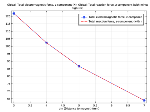
In the Settings window for Global, click Replace Expression in the upper-right corner of the y-Axis Data section. From the menu, choose Component 1 (comp1) > Magnetic Fields, No Currents > Mechanical > Electromagnetic force (spatial frame) - N > mfnc.Forcez_1 - Electromagnetic force, z-component.
|
|
3
|
Locate the y-Axis Data section. In the table, enter the following settings:
|
|
4
|
Locate the Coloring and Style section. Find the Line markers subsection. From the Marker list, choose Cycle.
|
|
1
|
|
2
|
In the Settings window for Global, click Replace Expression in the upper-right corner of the y-Axis Data section. From the menu, choose Component 1 (comp1) > Solid Mechanics > Reactions > Total reaction force (spatial frame) - N > solid.RFtotalz - Total reaction force, z-component.
|
|
3
|
Locate the y-Axis Data section. In the table, enter the following settings:
|
|
4
|
Locate the Coloring and Style section. Find the Line style subsection. From the Line list, choose Dashed.
|
|
5
|
|
6
|