|
|
|
|
1
|
|
2
|
In the Select Physics tree, select AC/DC > Electromagnetics and Mechanics > Magnetostriction > Piezomagnetism.
|
|
3
|
Click Add.
|
|
4
|
Click
|
|
5
|
|
6
|
Click
|
|
1
|
|
2
|
|
3
|
Click
|
|
4
|
Browse to the model’s Application Libraries folder and double-click the file piezomagnetic_cell_rover_parameters.txt.
|
|
1
|
|
2
|
|
3
|
|
1
|
|
2
|
|
3
|
|
4
|
|
5
|
|
6
|
|
7
|
|
8
|
Click to expand the Layers section. In the table, enter the following settings:
|
|
9
|
|
10
|
Clear the Bottom checkbox.
|
|
11
|
Locate the Selections of Resulting Entities section. Select the Resulting objects selection checkbox.
|
|
12
|
Click
|
|
1
|
|
2
|
|
3
|
|
4
|
|
5
|
Locate the Selections of Resulting Entities section. Select the Resulting objects selection checkbox.
|
|
6
|
Click
|
|
1
|
|
2
|
|
1
|
|
2
|
|
3
|
|
4
|
|
5
|
Click OK.
|
|
1
|
|
2
|
|
3
|
|
4
|
|
5
|
Click OK.
|
|
6
|
|
7
|
|
8
|
|
9
|
|
1
|
|
2
|
|
3
|
|
4
|
Click
|
|
5
|
|
6
|
Click OK.
|
|
1
|
|
2
|
|
3
|
|
4
|
|
1
|
|
2
|
Go to the Add Material window.
|
|
3
|
|
4
|
Click the Add to Component button in the window toolbar.
|
|
5
|
|
1
|
In the Model Builder window, under Component 1 (comp1) right-click Materials and choose Blank Material.
|
|
2
|
|
3
|
|
4
|
Click to expand the Material Properties section. In the Material properties tree, select Solid Mechanics > Linear Elastic Material > Young’s Modulus and Poisson’s Ratio.
|
|
5
|
Click
|
|
6
|
Locate the Material Contents section. In the table, enter the following settings:
|
|
1
|
|
2
|
|
3
|
|
4
|
|
5
|
|
6
|
|
1
|
In the Model Builder window, under Component 1 (comp1) > Magnetic Fields (mf) click Ampère’s Law, Piezomagnetic 1.
|
|
2
|
|
3
|
|
1
|
|
2
|
In the Settings window for External Magnetic Vector Potential, locate the Boundary Selection section.
|
|
3
|
|
1
|
|
2
|
|
3
|
|
1
|
|
2
|
Drag and drop below Initial Values 1.
|
|
3
|
|
4
|
Click
|
|
5
|
|
6
|
Click OK.
|
|
1
|
|
2
|
|
3
|
|
1
|
|
2
|
|
3
|
|
1
|
|
2
|
|
3
|
From the list, choose User-controlled mesh.
|
|
1
|
|
2
|
Drag and drop below Size 2.
|
|
3
|
|
4
|
|
5
|
|
1
|
|
2
|
|
3
|
Click the Custom button.
|
|
4
|
Locate the Element Size Parameters section.
|
|
5
|
|
6
|
|
7
|
|
8
|
|
1
|
|
2
|
|
3
|
|
1
|
|
2
|
|
1
|
|
2
|
|
3
|
|
4
|
|
5
|
|
1
|
|
2
|
|
3
|
In the Model Builder window, expand the Study 1 Frequency Domain > Solver Configurations > Solution 1 (sol1) > Stationary Solver 1 node.
|
|
4
|
Right-click Study 1 Frequency Domain > Solver Configurations > Solution 1 (sol1) > Stationary Solver 1 and choose Fully Coupled.
|
|
5
|
|
6
|
|
7
|
|
1
|
|
2
|
|
3
|
|
4
|
|
1
|
|
2
|
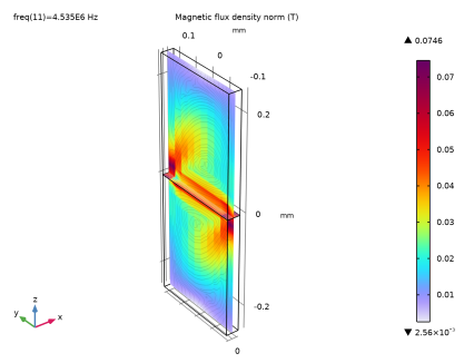
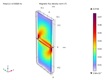
In the Settings window for 3D Plot Group, type Magnetic Flux Density Norm (mf) in the Label text field.
|
|
3
|
|
1
|
In the Model Builder window, expand the Magnetic Flux Density Norm (mf) node, then click Multislice 1.
|
|
2
|
|
3
|
|
4
|
|
1
|
|
2
|
|
3
|
|
4
|
|
1
|
|
2
|
|
3
|
|
4
|
|
5
|
|
1
|
|
2
|
|
3
|
|
4
|
|
5
|
|
1
|
|
2
|
|
3
|
|
4
|
|
5
|
|
6
|
|
1
|
|
2
|
|
3
|
|
1
|
|
2
|
|
1
|
|
2
|
|
1
|
|
2
|
|
3
|
Click
|
|
4
|
|
5
|
Click OK.
|
|
6
|
|
7
|
|
8
|
|
9
|
|
10
|
Click to expand the Coloring and Style section. Find the Line style subsection. From the Line list, choose Dashed.
|
|
11
|
|
12
|
|
13
|
|
1
|
|
2
|
|
1
|
|
2
|
Go to the Add Study window.
|
|
3
|
|
4
|
Click the Add Study button in the window toolbar.
|
|
1
|
In the Study toolbar, click
|
|
2
|
|
3
|
|
4
|
|
6
|
Click to expand the Store in Output section. In the table, enter the following settings:
|
|
7
|
|
8
|
|
9
|
Click OK.
|
|
10
|
|
11
|
|
12
|
|
13
|
|
1
|
|
2
|
|
3
|
|
4
|
|
5
|
|
6
|
Click OK.
|
|
7
|
|
8
|
|
9
|
|
10
|
|
11
|
|
12
|
|
13
|
|
1
|
|
2
|
|
3
|
|
4
|
|
5
|
Select the Include unit checkbox.
|
|
6
|
|
7
|
|
8
|