|
|
|
 |
 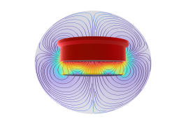 |

 relative permeability.
|
1
|
|
2
|
In the Select Physics tree, select AC/DC > Magnetic Fields, No Currents > Magnetic Fields, No Currents (mfnc).
|
|
3
|
Click Add.
|
|
4
|
Click
|
|
5
|
|
6
|
Click
|
|
1
|
|
2
|
|
3
|
|
1
|
|
2
|
|
3
|
|
4
|
Click to expand the Layers section. In the table, enter the following settings:
|
|
5
|
|
6
|
|
1
|
|
2
|
|
3
|
|
4
|
|
5
|
Click
|
|
6
|
Click
|
|
7
|
|
8
|
Locate the Selections of Resulting Entities section. Select the Resulting objects selection checkbox.
|
|
9
|
|
10
|
|
11
|
|
1
|
|
2
|
|
3
|
|
1
|
|
2
|
|
1
|
|
2
|
|
3
|
|
4
|
|
5
|
|
6
|
Click
|
|
1
|
|
2
|
On the object r1, select Point 2 only.
|
|
3
|
|
4
|
|
5
|
Click
|
|
1
|
|
2
|
|
3
|
|
4
|
|
5
|
|
1
|
In the Model Builder window, under Component 1 (comp1) > Geometry 1 right-click Work Plane 1 (wp1) and choose Revolve.
|
|
2
|
|
3
|
Locate the Selections of Resulting Entities section. Select the Resulting objects selection checkbox.
|
|
4
|
|
5
|
Click
|
|
1
|
|
2
|
|
3
|
Locate the Selections of Resulting Entities section. Select the Resulting objects selection checkbox.
|
|
4
|
|
5
|
Click
|
|
1
|
|
2
|
|
3
|
|
4
|
|
5
|
|
1
|
|
2
|
|
1
|
|
2
|
|
3
|
Click
|
|
4
|
In the Add dialog, in the Selections to invert list, choose Layer 1 (Sphere 1), Core (Sphere 1), Magnet, and Cap.
|
|
5
|
Click OK.
|
|
6
|
|
7
|
Click
|
|
8
|
|
9
|
|
10
|
|
11
|
|
12
|
Click
|
|
1
|
|
2
|
Go to the Add Material window.
|
|
3
|
|
4
|
Click the Add to Component button in the window toolbar.
|
|
1
|
|
2
|
|
1
|
Go to the Add Material window.
|
|
2
|
|
3
|
Click the Add to Component button in the window toolbar.
|
|
1
|
|
2
|
|
3
|
Locate the Material Contents section. In the table, enter the following settings:
|
|
1
|
Go to the Add Material window.
|
|
2
|
In the tree, select AC/DC > Hard Magnetic Materials > Sintered NdFeB Grades (Chinese Standard) > N28TH (Sintered NdFeB).
|
|
3
|
Click the Add to Component button in the window toolbar.
|
|
1
|
|
2
|
|
1
|
Go to the Add Material window.
|
|
2
|
|
3
|
Click the Add to Component button in the window toolbar.
|
|
1
|
|
2
|
|
3
|
|
4
|
Click to expand the Material Properties section. In the Material properties tree, select Basic Properties > Relative Permeability.
|
|
5
|
Click
|
|
6
|
Locate the Material Contents section. In the table, enter the following settings:
|
|
1
|
|
2
|
|
3
|
|
4
|
|
1
|
|
2
|
|
3
|
|
4
|
|
5
|
Specify the e vector as
|
|
1
|
|
2
|
|
3
|
|
4
|
|
1
|
|
1
|
|
2
|
|
3
|
|
4
|
|
1
|
|
2
|
|
3
|
|
4
|
|
1
|
|
2
|
|
3
|
|
4
|
|
5
|
|
6
|
|
7
|
From the list, choose Physics-controlled mesh.
|
|
8
|
|
1
|
|
2
|
|
3
|
|
1
|
|
2
|
|
1
|
|
2
|
|
3
|
|
4
|
|
1
|
|
2
|
|
3
|
|
4
|
|
5
|
|
1
|
|
2
|
|
3
|
|
4
|
|
5
|
|
1
|
|
2
|
|
3
|
|
4
|
|
1
|
|
2
|
|
3
|
|
4
|
Locate the Expressions section. In the table, enter the following settings:
|
|
5
|
|
1
|
|
2
|
|
1
|
|
2
|
|
3
|
|
1
|
|
2
|
|
3
|
Select the Modify model configuration for study step checkbox.
|
|
4
|
|
5
|
Right-click and choose Disable.
|
|
1
|
|
2
|
Go to the Add Study window.
|
|
3
|
|
4
|
Click the Add Study button in the window toolbar.
|
|
5
|
|
1
|
|
2
|
|
3
|
|
1
|
|
2
|
|
3
|
|
4
|
|
5
|
|
1
|
|
2
|
|
3
|
|
4
|
Locate the Expressions section. In the table, enter the following settings:
|
|
5
|
|
1
|
|
2
|
In the Settings window for Magnetic Shielding, type Nonlinear Shielding Alloy in the Label text field.
|
|
3
|
|
1
|
|
2
|
Go to the Add Study window.
|
|
3
|
|
4
|
Click the Add Study button in the window toolbar.
|
|
5
|
|
1
|
|
2
|
|
3
|
|
1
|
|
2
|
|
3
|
Select the Modify model configuration for study step checkbox.
|
|
4
|
In the tree, select Component 1 (comp1) > Magnetic Fields, No Currents (mfnc) > Nonlinear Shielding Alloy.
|
|
5
|
Right-click and choose Disable.
|
|
1
|
|
2
|
|
3
|
In the tree, select Component 1 (comp1) > Magnetic Fields, No Currents (mfnc) > Nonlinear Shielding Alloy.
|
|
4
|
Right-click and choose Disable.
|
|
1
|
|
2
|
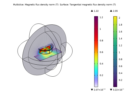
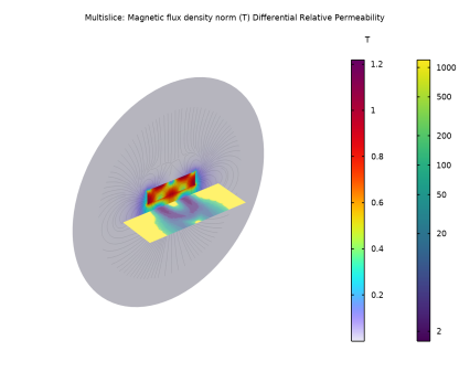
In the Settings window for 3D Plot Group, type One-sided Magnet - Nonlinear in the Label text field.
|
|
3
|
Locate the Data section. From the Dataset list, choose One-sided Magnet - Nonlinear/Solution 3 (sol3).
|
|
4
|
|
1
|
|
2
|
|
3
|
|
4
|
Locate the Expressions section. In the table, enter the following settings:
|
|
5
|
|
1
|
|
2
|
|
3
|
Clear the Transpose checkbox.
|
|
4
|
|
1
|
|
2
|
Select the Transpose checkbox.
|
|
3
|
|
1
|
|
2
|
In the Settings window for Surface, type Differential Relative Permeability in the Label text field.
|
|
3
|
|
4
|
Locate the Expression section. In the Expression text field, type d(comp1.mat4.BHCurve.BH(mfnc.ms2.normtHshield),mfnc.ms2.normtHshield)/mu0_const.
|
|
5
|
|
1
|
|
2
|
|
3
|
Clear the Show maximum and minimum values checkbox.
|
|
4
|
Select the Show units checkbox.
|
|
5
|
|
6
|