

PDF

Self-Inductance and Mutual Inductance of a Single Conductor and a Homogenized Helical Coil
Introduction
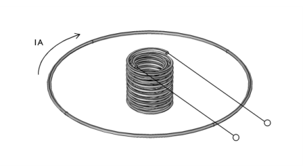
The mutual inductance and induced currents between a single-turn primary and 20-turn secondary coil in a concentric coplanar arrangement is computed using a frequency-domain model. The secondary coil is modeled using a homogenized approach, which does not explicitly consider each turn of the coil. Static and AC results are compared one against the other, and against analytic predictions.
Figure 1: A 20-turn secondary coil inside of a single-turn primary coil (not to scale).
Model Definition
The physical situation being modeled is shown in Figure 1. A secondary coil composed of 20 turns, wound two deep, is concentric with the primary, and in the same plane. The radius of the centroid of the secondary coil is R2 = 10 mm. The wire radii in both coils is r0 = mm. Although the coils are shown in 3D, they are modeled in the 2D axisymmetric space, assuming no physical variation around the centerline. First two DC analyses are solved in order to extract the inductance matrix of the system. Then a prescribed current of 1 A is flowing through a single-turn coil of radius R1 = 100 mm, at a frequency of 1 kHz. The objective of this is computing the voltage difference at the secondary coil for the open circuit case, and the induced currents for the closed circuit case.
For the case of a secondary multiturn coil with N turns, and in the limit as R1 >> R2 >> r0, the analytic expression for the mutual inductance between the two coils is:
where μ0 is the permeability of free space.
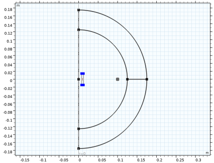
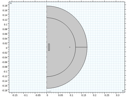
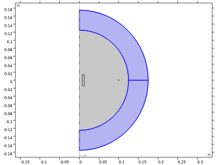
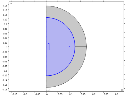
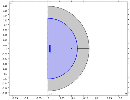
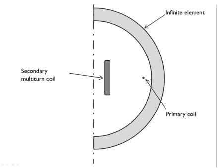
The two concentric coils are modeled in a 2D axisymmetric sense, as shown schematically in Figure 2. The individual turns of the secondary are not modeled. Rather, the secondary is modeled using a domain that describes the outside envelope of the coil. The modeling domain is surrounded by a region of Infinite Elements, which provide a way to truncate a domain that stretches to infinity. Although the thickness of the Infinite Element Domain is finite, it can be thought of as a domain of infinite extent.
Figure 2: A schematic representation of the 2D axisymmetric model of the concentric coils.
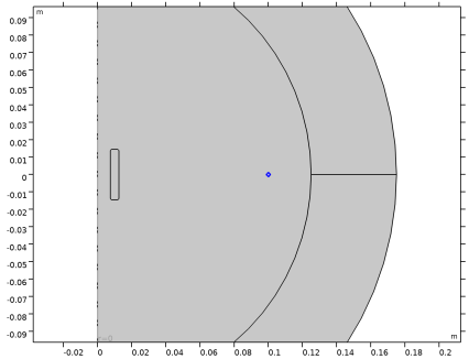
The primary coil is modeled using the Coil feature, which can be thought of as introducing an infinitesimal slit in an otherwise continuous torus. Since the coil has a single turn and is made up of conductive material, the Single conductor model is used in the Coil feature. The feature is used to excite the coil by specifying a current of 1 A.
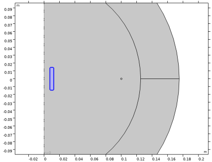
The secondary coil is modeled using another Coil feature using the Homogenized multiturn model, which treats the coil cross section as carrying a homogenized current that flows only in the circumferential direction. This feature can be used to model both the open circuit and the closed circuit case. To model the open circuit case, the current through the coil is specified to be 0 A, which specifies that there is no current flowing through the coil. To model a closed circuit it is enough to put 0 V. The Coil feature computes the total current and potential drop on the entire coil. Furthermore, if just one coil only is fed, also self-inductance and mutual inductance of the coil system are available in the output. For AC feeding, assuming the system to be purely reactive, mutual inductance can be computed via:
(1)
Where ω is the angular frequency of excitation of the driving current in the primary coil, Ip. The inductance computed in this fashion will have a small imaginary component. More explicitly, due to finite conductivity, there are eddy current losses in the wires and the coil impedance, though mainly reactive, has a small resistive part. The deduced inductance is compared against the inductance predicted by taking the integral of the magnetic flux through the center of the coil.
To model the closed circuit case, the applied voltage across the coil feed is fixed at 0 V which is analogous to a coil with a shorted feed gap. That is, a closed continuous loop of wire. DC resistance of the homogenized coil is included as well as impedance. These effects, however, cannot describe skin and proximity effect which need the Coil Group approach (losses due to these effects are sometimes called additional losses).
In a simple circuital analogy, and for frequencies such that the skin depth is significantly larger than the conductor size, this current can be estimated from DC values via:
(2)
where L21 is mutual inductance and is the impedance of the inner coil. At the simulated 1 kHz deviations are really small. Increasing the frequency, this estimate will fail as the model is able to capture the autoinductance effects on the coil that are not included in the simplest circuital analogy.

Results and Discussion
From two initial static analyses one feeding the single coil, the other feeding the 20-turn coil group, it is possible to extract from built in variables the following inductance matrix:
A similar estimate is extracted by computing the integral of the normal magnetic flux. This approach is generally less accurate, since the result depends more strongly on the mesh resolution and interpolation of the magnetic field.
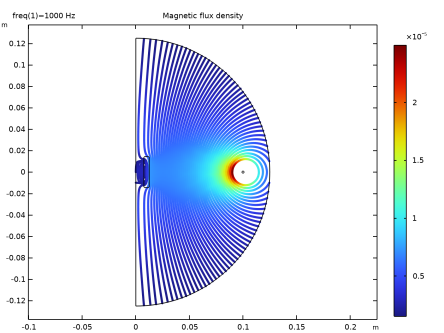
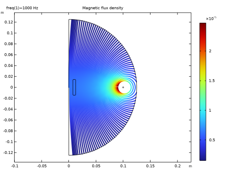
In the case of an AC feeding the primary coil, the magnetic flux lines are plotted in Figure 3 for the open circuit case. The Coil feature computes the voltage across the secondary coil, which can be used to evaluate the mutual inductance, 40.0 nH. This agrees well with the mutual inductance predicted by static calculations and with the analytic mutual inductance estimate of 39.478 nH
The magnetic flux lines are plotted in Figure 4 for the closed circuit case. The induced current through the secondary coil is 10.7  3.3i mA, the imaginary component implies a reactive current. These results also agree well with the Coil Group approach. Both real and imaginary parts are correctly accounted by Equation 2.
Figure 3: Magnetic flux lines for the open circuit case.
Figure 4: Magnetic flux lines for the closed circuit case.
Application Library path: ACDC_Module/Tutorials,_Coils/mutual_inductance_multiturn
Modeling Instructions
From the File menu, choose New.
New
In the New window, click  Model Wizard.
Model Wizard
1
In the Model Wizard window, click  2D Axisymmetric.
2
In the Select Physics tree, select AC/DC > Electromagnetic Fields > Magnetic Fields (mf).
3
Click Add.
4
Click  Study.
5
In the Select Study tree, select General Studies > Stationary.
6
Global Definitions
Parameters 1
1
In the Model Builder window, under Global Definitions click Parameters 1.
2
In the Settings window for Parameters, locate the Parameters section.
3
Here, mu0_const a predefined COMSOL constant for the permeability in vacuum.
Geometry 1
Create a circle for the simulation domain. Define layer in the circle where you will assign the Infinite Element Domain.
Circle 1 (c1)
1
In the Geometry toolbar, click  Circle.
2
In the Settings window for Circle, locate the Size and Shape section.
3
In the Sector angle text field, type 180.
4
In the Radius text field, type 1.75*R1.
5
Locate the Rotation Angle section. In the Rotation text field, type -90.
6
Click to expand the Layers section. In the table, enter the following settings:
Create a circle for the outer coil.
Circle 2 (c2)
1
In the Geometry toolbar, click  Circle.
2
In the Settings window for Circle, locate the Size and Shape section.
3
In the Radius text field, type r_wire.
4
Locate the Position section. In the r text field, type R1.
Create a rectangle where you will assign the coil properties.
Rectangle 1 (r1)
1
In the Geometry toolbar, click  Rectangle.
2
In the Settings window for Rectangle, locate the Size and Shape section.
3
In the Width text field, type r_wire*5.
4
In the Height text field, type r_wire*29.
5
Locate the Position section. From the Base list, choose Center.
6
In the r text field, type R2.
Fillet 1 (fil1)
1
In the Geometry toolbar, click  Fillet.
2
On the object r1, select Points 1–4 only.
3
In the Settings window for Fillet, locate the Radius section.
4
In the Radius text field, type r_wire.
5
Click  Build All Objects.
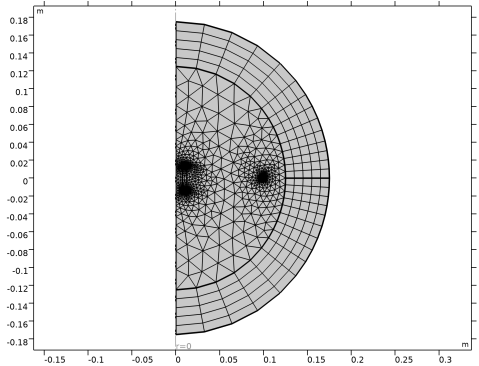
Define the Infinite Element Domain where you truncate the domain which stretches to infinity. The Physics-Controlled Mesh creates a Swept mesh inside the Infinite Elements domains.
Definitions
Infinite Element Domain 1 (ie1)
1
In the Definitions toolbar, click  Infinite Element Domain.
2
Magnetic Fields (mf)
Now, set up the physics. Assign a Coil feature on the outer and the inner coil. The outer coil will be initially fed with a current of 1 A.
1
Click the  Zoom In button in the Graphics toolbar.
Domain Coil 1
1
In the Physics toolbar, click  Domains and choose Domain Coil.
2
In the Settings window for Domain Coil, locate the Coil section.
3
In the Icoil text field, type I1.
4
Specify 0 A current for the Coil feature assigned to the inner coil to model the open circuit case.
Domain Coil 2
1
In the Physics toolbar, click  Domains and choose Domain Coil.
2
3
In the Settings window for Domain Coil, locate the Coil section.
4
From the Conductor model list, choose Homogenized multiturn.
5
In the Icoil text field, type I2.
6
Locate the Homogenized Conductor section. In the N text field, type N.
7
From the Coil wire cross-section area list, choose User defined.
8
Find the High-frequency effective loss subsection. Clear the Include harmonic loss checkbox.
9
In the a text field, type pi*r_wire^2.
Materials
Next, assign material properties. Use Air for all domains.
Add Material
1
In the Materials toolbar, click  Add Material to open the Add Material window.
2
Go to the Add Material window.
3
In the tree, select Built-in > Air.
4
Click the Add to Component button in the window toolbar.
Materials
Air (mat1)
Then, override the outer coil domain with copper.
Add Material
1
Go to the Add Material window.
2
In the tree, select AC/DC > Copper.
3
Click the Add to Component button in the window toolbar.
4
In the Materials toolbar, click  Add Material to close the Add Material window.
Materials
Copper (mat2)
1
2
Click the  Zoom Extents button in the Graphics toolbar.
Mesh 1
In the Model Builder window, under Component 1 (comp1) right-click Mesh 1 and choose Build All.
Solve the first case where the outer coil (named 1) is fed and the inner (named 2) is open.
Study 1
1
In the Model Builder window, click Study 1.
2
In the Settings window for Study, locate the Study Settings section.
3
Clear the Generate default plots checkbox.
4
In the Study toolbar, click  Compute.
Results
In the Model Builder window, expand the Results node.
Study 1/Solution 1 (sol1)
Select only the domains not part of the Infinite Element Domain for better magnetic flux visualization.
1
In the Model Builder window, expand the Results > Datasets node, then click Study 1/Solution 1 (sol1).
Selection
1
In the Results toolbar, click  Attributes and choose Selection.
2
In the Settings window for Selection, locate the Geometric Entity Selection section.
3
From the Geometric entity level list, choose Domain.
4
2D Plot Group 1
In the Results toolbar, click  2D Plot Group.
Streamline 1
1
Right-click 2D Plot Group 1 and choose Streamline.
2
In the Settings window for Streamline, locate the Streamline Positioning section.
3
From the Positioning list, choose Starting-point controlled.
4
From the Entry method list, choose Coordinates.
5
In the r text field, type range(0,0.9*R1/49,0.9*R1).
6
In the z text field, type 0.
7
Locate the Coloring and Style section. Find the Line style subsection. From the Type list, choose Tube.
Color Expression 1
Right-click Streamline 1 and choose Color Expression.
Evaluate the self inductance of the external coil and the mutual inductance of the outer coil with respect to the inner. Some additional quantities are also computed to verify the results.
Global Evaluation 1
1
In the Results toolbar, click  Global Evaluation.
2
In the Settings window for Global Evaluation, locate the Expressions section.
3
4
Click  Evaluate.
Next, compute the self inductance of the inner coil and the mutual inductance of the inner coil with respect to the outer. Start by switching the currents in the coils.
Global Definitions
Parameters 1
1
In the Model Builder window, under Global Definitions click Parameters 1.
2
In the Settings window for Parameters, locate the Parameters section.
3
Now add and solve a second study for this case. The solution previously computed will still be available in Study 1.
Add Study
1
In the Home toolbar, click  Add Study to open the Add Study window.
2
Go to the Add Study window.
3
Find the Studies subsection. In the Select Study tree, select General Studies > Stationary.
4
Click the Add Study button in the window toolbar.
5
In the Home toolbar, click  Add Study to close the Add Study window.
Study 2
1
In the Settings window for Study, locate the Study Settings section.
2
Clear the Generate default plots checkbox.
3
In the Study toolbar, click  Compute.
The quantities of interest are evaluated in the following steps.
Results
Global Evaluation 2
1
In the Results toolbar, click  Global Evaluation.
2
In the Settings window for Global Evaluation, locate the Data section.
3
From the Dataset list, choose Study 2/Solution 2 (sol2).
4
Locate the Expressions section. In the table, enter the following settings:
5
Clicknext to  Evaluate, then choose New Table.
Table 2
1
Go to the Table 2 window.
Self and mutual inductance variables as computed above are derived via concatenated flux, which is defined as the line integral of the magnetic vector potential along the coil. This approach gives the best accuracy.
For simple geometries like the present one, concatenated flux can be also computed explicitly using its definition as the integral of magnetic flux through a surface, although this approach usually gives less accurate results.
Results
Cut Line 2D 1
1
In the Results toolbar, click  Cut Line 2D.
2
In the Settings window for Cut Line 2D, locate the Line Data section.
3
In row Point 2, set r to R2.
Cut Line 2D 2
1
In the Results toolbar, click  Cut Line 2D.
2
In the Settings window for Cut Line 2D, locate the Line Data section.
3
In row Point 2, set r to R1.
Line Integration 1
1
In the Results toolbar, click  More Derived Values and choose Integration > Line Integration.
2
In the Settings window for Line Integration, locate the Data section.
3
From the Dataset list, choose Cut Line 2D 1.
4
Locate the Expressions section. In the table, enter the following settings:
5
Clicknext to  Evaluate, then choose New Table.
Line Integration 2
1
Right-click Line Integration 1 and choose Duplicate.
2
In the Settings window for Line Integration, locate the Data section.
3
From the Dataset list, choose Cut Line 2D 2.
4
Locate the Expressions section. In the table, enter the following settings:
5
Clicknext to  Evaluate, then choose Table 3 - Line Integration 1.
Cut Line 2D 1
1
In the Model Builder window, under Results > Datasets click Cut Line 2D 1.
2
In the Settings window for Cut Line 2D, locate the Data section.
3
From the Dataset list, choose Study 2/Solution 2 (sol2).
Cut Line 2D 2
1
In the Model Builder window, click Cut Line 2D 2.
2
In the Settings window for Cut Line 2D, locate the Data section.
3
From the Dataset list, choose Study 2/Solution 2 (sol2).
Line Integration 1
1
In the Model Builder window, under Results > Derived Values click Line Integration 1.
2
In the Settings window for Line Integration, locate the Expressions section.
3
4
Clicknext to  Evaluate, then choose Table 3 - Line Integration 1.
Line Integration 2
1
In the Model Builder window, click Line Integration 2.
2
In the Settings window for Line Integration, locate the Expressions section.
3
4
Clicknext to  Evaluate, then choose Table 3 - Line Integration 1.
Experimentally, mutual inductance is measured by feeding an AC signal in the primary coil and measuring the voltage induced in the open-circuit secondary coil. This procedure can be simulated by using a Frequency Domain study step. Start by setting the AC feed on Coil 1 and the open circuit (zero current) condition on Coil 2.
Global Definitions
Parameters 1
1
In the Model Builder window, under Global Definitions click Parameters 1.
2
In the Settings window for Parameters, locate the Parameters section.
3
Add Study
1
In the Home toolbar, click  Add Study to open the Add Study window.
2
Go to the Add Study window.
3
Find the Studies subsection. In the Select Study tree, select General Studies > Frequency Domain.
4
Click the Add Study button in the window toolbar.
5
In the Home toolbar, click  Add Study to close the Add Study window.
Study 3
Step 1: Frequency Domain
1
In the Settings window for Frequency Domain, locate the Study Settings section.
2
In the Frequencies text field, type 1[kHz].
3
In the Model Builder window, click Study 3.
4
In the Settings window for Study, locate the Study Settings section.
5
Clear the Generate default plots checkbox.
6
In the Study toolbar, click  Compute.
Results
Study 3/Solution 3 (sol3)
Select the inner coil domains.
1
In the Model Builder window, under Results > Datasets click Study 3/Solution 3 (sol3).
Selection
1
In the Results toolbar, click  Attributes and choose Selection.
2
In the Settings window for Selection, locate the Geometric Entity Selection section.
3
From the Geometric entity level list, choose Domain.
4
2D Plot Group 1
1
In the Model Builder window, under Results click 2D Plot Group 1.
2
In the Settings window for 2D Plot Group, locate the Data section.
3
From the Dataset list, choose Study 3/Solution 3 (sol3).
4
Click the  Zoom Extents button in the Graphics toolbar.
Compare the plot with Figure 3 describing the induced currents in the coil for the open circuit case.
Evaluate the mutual inductance using Equation 1 .
Global Evaluation 3
1
In the Results toolbar, click  Global Evaluation.
2
In the Settings window for Global Evaluation, locate the Data section.
3
From the Dataset list, choose Study 3/Solution 3 (sol3).
4
Locate the Expressions section. In the table, enter the following settings:
5
Click  Evaluate.
Finally, simulate the system as it were a transformer with a short-circuited secondary winding. Specify a voltage of 0 V for the Coil feature assigned to the inner coil to model the short-circuit condition.
Magnetic Fields (mf)
Domain Coil 2
1
In the Model Builder window, under Component 1 (comp1) > Magnetic Fields (mf) click Domain Coil 2.
2
In the Settings window for Domain Coil, locate the Coil section.
3
From the Coil excitation list, choose Voltage.
4
In the Vcoil text field, type 0.
Add Study
1
In the Home toolbar, click  Add Study to open the Add Study window.
2
Go to the Add Study window.
3
Find the Studies subsection. In the Select Study tree, select General Studies > Frequency Domain.
4
Click the Add Study button in the window toolbar.
5
In the Home toolbar, click  Add Study to close the Add Study window.
Study 4
Step 1: Frequency Domain
1
In the Settings window for Frequency Domain, locate the Study Settings section.
2
In the Frequencies text field, type 1[kHz].
3
In the Model Builder window, click Study 4.
4
In the Settings window for Study, locate the Study Settings section.
5
Clear the Generate default plots checkbox.
6
In the Study toolbar, click  Compute.
Results
Study 4/Solution 4 (sol4)
Select the inner coil domains.
1
In the Model Builder window, under Results > Datasets click Study 4/Solution 4 (sol4).
Selection
1
In the Results toolbar, click  Attributes and choose Selection.
2
In the Settings window for Selection, locate the Geometric Entity Selection section.
3
From the Geometric entity level list, choose Domain.
4
2D Plot Group 2
1
In the Results toolbar, click  2D Plot Group.
2
In the Settings window for 2D Plot Group, locate the Data section.
3
From the Dataset list, choose Study 4/Solution 4 (sol4).
Streamline 1
1
Right-click 2D Plot Group 2 and choose Streamline.
2
In the Settings window for Streamline, locate the Streamline Positioning section.
3
From the Positioning list, choose Starting-point controlled.
4
From the Entry method list, choose Coordinates.
5
In the r text field, type range(0,0.9*R1/49,0.9*R1).
6
In the z text field, type 0.
7
Locate the Coloring and Style section. Find the Line style subsection. From the Type list, choose Tube.
Color Expression 1
1
Right-click Streamline 1 and choose Color Expression.
2
Click the  Zoom Extents button in the Graphics toolbar.
Compare the plot with Figure 4 describing the induced currents in the coil for the closed circuit case.
Evaluate the total induced current on the inner (secondary) coil. This quantity is related to static quantities, being in the simplest approximation iωM/(R2 + iωL2) times 1[A] .
Global Evaluation 4
1
In the Results toolbar, click  Global Evaluation.
2
In the Settings window for Global Evaluation, locate the Data section.
3
From the Dataset list, choose Study 4/Solution 4 (sol4).
4
Locate the Expressions section. In the table, enter the following settings:
5
Click  Evaluate.