COMSOL 6.4 - Multiturn Coil Above an Asymmetric Conductor Plate

Multiturn Coil Above an Asymmetric Conductor Plate

This model solves the Testing Electromagnetic Analysis Methods (TEAM) problem 7, “Asymmetrical Conductor with a Hole” — a benchmark problem concerning the calculation of eddy currents and magnetic fields produced when an aluminum conductor is placed asymmetrically above a multiturn coil carrying a sinusoidally varying current. The simulation results at specified positions in space are compared with measured data from the literature and agreement is shown.

Figure 1: A multiturn coil placed asymmetrically over an aluminum plate with a hole.

Model Definition

Because the geometry has no symmetries, the problem must be solved for the entire geometry. As shown in Figure 1, the geometry consists of a coil placed asymmetrically above a thick aluminum conductor with an eccentric square hole. The coil has 2742 turns and carries a sinusoidally varying current of 1 A/turn. The magnetic field and the eddy currents induced in the conductor for coil currents of frequencies 50 Hz and 200 Hz are calculated, and the simulation results along specified locations in space are compared with experimental data given in Ref. 1.

Results and Discussion

Figure 2 visualizes the induced current at 50 Hz using a combined surface and arrow plot. The black arrows show the current density in the conductor while the red arrows indicate the coil current direction is shown. Figure 3 shows the corresponding results at 200 Hz.

Figure 2: A 3D surface plot of the y-component of the induced current density, Jy (A/m2) in the conductor combined with the arrow volume plots of the coil current direction and the induced current density in the conductor. This simulation results are at 50 Hz.

Figure 3: A 3D surface plot of the y-component of the induced current density in the conductor combined with the arrow volume plots of the coil current direction and the induced current density in the conductor. This simulation results are at 200 Hz.

Figure 4 and Figure 5 show comparisons between the simulation and the measured data. In Figure 4, the z-component of the magnetic flux density, Bz (SI unit: mT), at 50 Hz and 200 Hz are compared with measured data from Ref. 1. These results are compared for 0 ≤ x ≤ 288 mm at y = 72 mm and z = 34 mm (a line between the aluminum plate and the copper coil). In Figure 5, similarly, the y-component values of the induced current density, Jy (SI unit: A/m2) at 50 Hz and 200 Hz are compared with the corresponding measured data. This is done at 0 ≤ x ≤ 288 mm, y = 72 mm, and z = 19 mm (a line on the surface of the aluminum plate that crosses the gap). As is evident from the plots, there is close agreement between the simulation results and the measured data.

Figure 4: z-component of the flux density, Bz (mT), at 0 ≤ x ≤ 288 mm, y = 72 mm, and z = 34 mm for 50 Hz and 200 Hz. The solid lines are simulation results while the circles are the corresponding measured data from Ref. 1.

Figure 5: y-components of the induced current densities, Jy (A/m2) for 0 ≤ x ≤ 288 mm at y = 72 mm, z = 19 mm for 50 Hz and 200 Hz. The solid lines are simulation results while the circles are the corresponding measured data from Ref. 1.

Notes About the COMSOL Implementation

The direction of the wires in the coil is computed using a Coil feature combined with a Coil Geometry Analysis study step. The eddy currents and the nonuniform magnetic field are computed using a Frequency Domain study step for the frequencies 50 Hz and 200 Hz.

Reference

1. K. Fujiwara and T. Nakata, “Results for Benchmark Problem 7 (Asymmetrical Conductor with a Hole),” Int. J. Comput. and Math. in Electr. and Electron. Eng., vol. 9, no. 3, pp. 137–154, 1990.

ACDC_Module/Verifications/multiturn_coil_asymmetric_conductor

Modeling Instructions

From the menu, choose .

New

In the window, click

Model Wizard

In the window, click

In the tree, select > > .

Click .

Click

In the tree, select .

Click

Geometry 1

Insert the geometry sequence provided in a separate file.

In the toolbar, click and choose .

Browse to the model’s Application Libraries folder and double-click the file multiturn_coil_asymmetric_conductor_geom_sequence.mph.

In the toolbar, click

Click the

button in the toolbar.

The model geometry is now complete.

Click the

button in the toolbar to get a better view of the interior parts.

In the window, under click .

Conductor

Define domain and boundary selections for the coil and the conductor.

In the window, under > click .

In the window for , type Conductor in the text field.

Locate the section. Select the checkbox.

Coil

In the window, under > click .

In the window for , type Coil in the text field.

Locate the section. Select the checkbox.

Hide the outer geometry boundaries to visualize the results only in the coil and the conductor domains.

Click the

button in the toolbar.

In the window toolbar, click

next to

, then choose .

Select the exterior boundaries of the block (Boundaries 1–5 and 52).

Click the

button in the toolbar.

Click the

button in the toolbar.

Magnetic Fields (mf)

Now set up the physics. Start by setting to the aluminum plate.

Ampère’s Law in Solids 1

In the toolbar, click

and choose .

In the window for , locate the section.

From the list, choose .

In the window, right-click and choose .

Click the

button in the toolbar.

Domain Coil 1

In the toolbar, click

and choose .

In the window for , locate the section.

From the list, choose .

Locate the section. From the list, choose .

Locate the section. In the N text field, type 2742.

Apply the input on a cross-sectional coil boundary.

Input 1

In the window, expand the > > > > node, then click .

Select Boundary 37 only.

Materials

Add material for the components.

Add Material

In the toolbar, click

to open the window.

Go to the window.

In the tree, select > .

Click the button in the window toolbar.

In the toolbar, click

to close the window.

Materials

Copper (mat1)

In the window for , locate the section.

From the list, choose .

Create a new material for the conductor. This will have the relevant properties of Aluminum

Aluminum

In the window, right-click and choose .

In the window for , locate the section.

From the list, choose .

Locate the section. In the table, enter the following settings:


Property	Variable	Value	Unit	Property group
Relative permeability	mur_iso ; murii = mur_iso, murij = 0	1	1	Basic
Electric conductivity	sigma_iso ; sigmaii = sigma_iso, sigmaij = 0	3.526e7	S/m	Basic
Relative permittivity	epsilonr_iso ; epsilonrii = epsilonr_iso, epsilonrij = 0	1	1	Basic

In the text field, type Aluminum.

Mesh 1

Use a finer mesh in the aluminum plate to better resolve the eddy currents and obtain a more accurate solution.

Size 1

In the window, under right-click and choose .

In the window for , locate the section.

From the list, choose .

Locate the section. Click the button.

Locate the section.

Select the checkbox. In the associated text field, type 12.

Size 2

In the window, right-click and choose .

In the window for , locate the section.

From the list, choose .

Locate the section. Click the button.

Locate the section.

Select the checkbox. In the associated text field, type 20.

Free Tetrahedral 1

In the toolbar, click

In the window for , click

The mesh should look like that shown in the figure below.

Study 1

Next, set up the study. Start by adding a preprocessing study step before the Frequency Domain step.

Step 1: Coil Geometry Analysis

In the toolbar, click

and choose > .

This study step computes the direction of the wires in the coils.

Add the main Frequency Domain study step. Solve the problem in the frequency domain for 50 Hz and 200 Hz.

Step 2: Frequency Domain

In the toolbar, click

In the window for , locate the section.

In the text field, type 50 200.

In the window, click .

In the window for , locate the section.

Clear the checkbox.

In the toolbar, click

Results

To reproduce the plot shown in Figure 2, create a 3D plot group and add an Arrow Volume plot of the coil current direction in the coil domain, computed by the Coil Geometry Analysis step. Add an Arrow Volume plot of the induced current on the conductor surface and a Volume plot of the y component of the induced current density to the same plot group.

Coil Direction and Induced Current Density, 50 Hz

In the window, expand the node.

Right-click and choose .

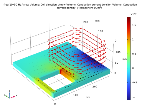
In the window for , type Coil Direction and Induced Current Density, 50 Hz in the text field.

Locate the section. From the list, choose .

Arrow Volume 1

Right-click and choose .

Selection 1

In the window, right-click and choose .

In the window for , locate the section.

From the list, choose .

Arrow Volume 1

In the window, click .

In the window for , click in the upper-right corner of the section. From the menu, choose > > > .

Locate the section. Find the subsection. In the text field, type 10.

Find the subsection. In the text field, type 10.

Find the subsection. In the text field, type 5.

Locate the section.

Select the checkbox. In the associated text field, type 20.

Arrow Volume 2

In the window, right-click and choose .

Selection 1

In the window, right-click and choose .

In the window for , locate the section.

From the list, choose .

Arrow Volume 2

In the window, click .

In the window for , click in the upper-right corner of the section. From the menu, choose > > > .

Locate the section. Find the subsection. In the text field, type 20.

Find the subsection. In the text field, type 20.

Find the subsection. From the list, choose .

In the text field, type 19.

Locate the section. From the list, choose .

From the list, choose .

Volume 1

In the window, right-click and choose .

Selection 1

In the window, right-click and choose .

In the window for , locate the section.

From the list, choose .

Volume 1

In the window, click .

In the window for , click in the upper-right corner of the section. From the menu, choose > > > > .

Coil Direction and Induced Current Density, 50 Hz

In the window, click .

In the window for , locate the section.

Clear the checkbox.

In the toolbar, click

Duplicate the plot group just created and modify the copy to generate the plot shown in Figure 3. This figure is similar to the Figure 2 except the frequency is 200 Hz.

Coil Direction and Induced Current Density, 200 Hz

Right-click and choose .

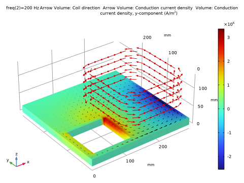
In the window for , type Coil Direction and Induced Current Density, 200 Hz in the text field.

Locate the section. From the list, choose .

In the toolbar, click

To generate the plots shown in Figure 4 and Figure 5, begin by creating two cut line datasets.

Cut Line 3D 1

In the toolbar, click

In the window for , locate the section.

In row , set to 72 and to 34.

In row , set to 288, to 72, and to 34.

Cut Line 3D 2

Right-click and choose .

Specify a value of z slightly below the surface of the conductor.

In the window for , locate the section.

In row , set to 18.99.

Import the experimental data of Bz and Jy in two tables.

Table 1

In the toolbar, click

In the window for , locate the section.

Click

Browse to the model’s Application Libraries folder and double-click the file multiturn_coil_asymmetric_conductor_table1.txt.

Locate the section. In the table, enter the following settings:


Column	Header
1	x [mm]
2	Bz(x,72,34) at 50Hz
3	Bz(x,72,34) at 200Hz

Table 2

In the toolbar, click

In the window for , locate the section.

Click

Browse to the model’s Application Libraries folder and double-click the file multiturn_coil_asymmetric_conductor_table2.txt.

Locate the section. In the table, enter the following settings:


Column	Header
1	x [mm]
2	Jy(x,72,19) at 50Hz
3	Jy(x,72,19) at 200Hz

Plot the z-component of the magnetic flux density, Bz, along the lines defined by the cut line datasets just created.

1D Plot Group 3

In the toolbar, click

Line Graph 1

Right-click and choose .

In the window for , locate the section.

From the list, choose .

Locate the section. In the text field, type sign(real(mf.Bz))*abs(mf.Bz).

From the list, choose .

Click to expand the section. Select the checkbox.

From the list, choose .

In the text field, type eval(freq) Hz.

Bz(x,72,34)

Add a plot for the experimental value of Bz at 50 Hz to the same plot group using a table graph.

In the window, under click .

In the window for , type Bz(x,72,34) in the text field.

Table Graph 1

Right-click and choose .

In the window for , locate the section.

From the list, choose .

In the list box, select .

Locate the section. Find the subsection. From the list, choose .

From the list, choose .

Find the subsection. From the list, choose .

Duplicate the table graph previously created and modify to plot the experimental value of Bz at 200 Hz.

Table Graph 2

Right-click and choose .

In the window for , locate the section.

In the list box, select .

Locate the section. From the list, choose .

In the toolbar, click

Compare the resulting plot with that in Figure 4.

Plot the y-component of the current density on the surface of the conductor, Jy, along the line specified earlier. Use an approach similar to the one used to generate Figure 4.

1D Plot Group 4

In the toolbar, click