|
|
|


|
1
|
|
2
|
In the Select Physics tree, select AC/DC > Electromagnetics and Fluids > Magnetohydrodynamics, Out-of-Plane Currents.
|
|
3
|
Click Add.
|
|
4
|
Click
|
|
5
|
|
6
|
Click
|
|
1
|
|
2
|
|
1
|
|
2
|
|
3
|
|
4
|
|
1
|
|
2
|
|
3
|
|
4
|
|
5
|
|
6
|
Click to expand the Layers section. In the table, enter the following settings:
|
|
7
|
Select the Layers to the right checkbox.
|
|
8
|
Clear the Layers on bottom checkbox.
|
|
9
|
Click
|
|
1
|
|
2
|
|
3
|
|
4
|
|
5
|
|
6
|
Click
|
|
1
|
|
2
|
|
3
|
|
4
|
|
5
|
|
6
|
|
7
|
Click
|
|
1
|
|
2
|
|
3
|
|
4
|
|
5
|
|
6
|
|
7
|
Click
|
|
1
|
|
2
|
Select the object r4 only.
|
|
3
|
|
4
|
|
5
|
Click
|
|
1
|
|
2
|
Select the object r4 only.
|
|
3
|
|
4
|
|
5
|
|
1
|
|
3
|
|
4
|
|
1
|
|
2
|
|
3
|
Click
|
|
1
|
|
2
|
Go to the Add Material window.
|
|
3
|
|
4
|
Click the Add to Component button in the window toolbar.
|
|
1
|
|
2
|
|
4
|
Locate the Material Contents section. In the table, enter the following settings:
|
|
1
|
Go to the Add Material window.
|
|
2
|
|
3
|
Click the Add to Component button in the window toolbar.
|
|
4
|
|
1
|
In the Model Builder window, under Component 1 (comp1) > Magnetic Fields (mf) click Ampère’s Law in Fluids 1.
|
|
1
|
|
1
|
|
2
|
|
3
|
Click
|
|
4
|
|
5
|
Click OK.
|
|
1
|
|
2
|
|
3
|
|
4
|
|
5
|
Click OK.
|
|
6
|
|
7
|
|
8
|
|
9
|
|
1
|
|
2
|
|
3
|
|
5
|
|
1
|
|
2
|
|
3
|
|
5
|
|
1
|
|
2
|
|
3
|
Click
|
|
4
|
|
5
|
Click OK.
|
|
1
|
|
2
|
|
3
|
Click
|
|
4
|
|
5
|
Click OK.
|
|
1
|
In the Model Builder window, under Component 1 (comp1) > Multiphysics click Magnetohydrodynamics 1 (mhd1).
|
|
2
|
|
3
|
Click
|
|
1
|
|
2
|
|
3
|
From the list, choose User-controlled mesh.
|
|
1
|
|
2
|
|
3
|
|
4
|
Click
|
|
1
|
|
2
|
|
3
|
|
4
|
Click
|
|
1
|
|
2
|
|
3
|
Click
|
|
4
|
Click
|
|
5
|
|
6
|
Click OK.
|
|
7
|
|
8
|
|
9
|
|
10
|
Select the Symmetric distribution checkbox.
|
|
11
|
Click
|
|
1
|
|
2
|
|
3
|
|
5
|
|
1
|
|
2
|
|
3
|
|
1
|
|
3
|
Click
|
|
5
|
Click
|
|
1
|
|
2
|
|
3
|
|
4
|
Click
|
|
1
|
|
2
|
|
3
|
|
4
|
|
5
|
Click
|
|
8
|
|
9
|
|
1
|
|
2
|
|
3
|
In the Model Builder window, expand the Study 1 > Solver Configurations > Solution 1 (sol1) > Stationary Solver 1 node.
|
|
4
|
Right-click Study 1 > Solver Configurations > Solution 1 (sol1) > Stationary Solver 1 and choose Segregated.
|
|
5
|
In the Model Builder window, expand the Study 1 > Solver Configurations > Solution 1 (sol1) > Stationary Solver 1 > Segregated 1 node, then click Segregated Step.
|
|
6
|
|
7
|
|
8
|
|
9
|
In the Model Builder window, under Study 1 > Solver Configurations > Solution 1 (sol1) > Stationary Solver 1 right-click Segregated 1 and choose Segregated Step.
|
|
10
|
|
11
|
|
12
|
|
13
|
Click OK.
|
|
14
|
|
15
|
|
16
|
|
1
|
In the Model Builder window, expand the Results > Datasets node, then click Study 1/Solution 1 (sol1).
|
|
2
|
|
3
|
|
1
|
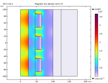
In the Model Builder window, expand the Results > Magnetic Flux Density (mf) node, then click Magnetic Flux Density (mf).
|
|
2
|
|
3
|
|
1
|
|
2
|
|
3
|
|
1
|
|
2
|
Select the Show maximum and minimum values checkbox.
|
|
3
|
|
4
|
|
1
|
|
2
|
|
3
|
Select the Show maximum and minimum values checkbox.
|
|
4
|
|
5
|
|
1
|
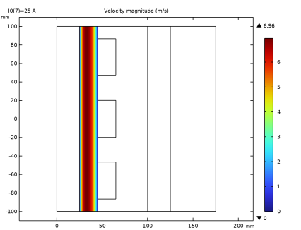
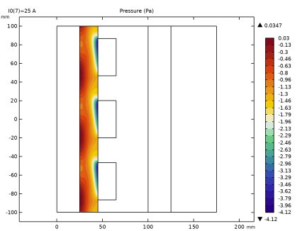
In the Model Builder window, expand the Pressure (spf) node, then click Results > Velocity, 3D (spf).
|
|
2
|
|
3
|
|
4
|
|
5
|
|
1
|
|
2
|
|
3
|
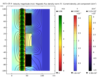
In the Settings window for 2D Plot Group, type Velocity and Magnetic Flux Density in the Label text field.
|
|
4
|
|
5
|
|
6
|
Select the Show units checkbox.
|
|
1
|
|
2
|
|
3
|
|
4
|
|
5
|
|
6
|
|
7
|
Clear the Color legend checkbox.
|
|
8
|
|
1
|
In the Model Builder window, right-click Velocity and Magnetic Flux Density and choose Arrow Surface.
|
|
2
|
|
3
|
|
4
|
Click Replace Expression in the upper-right corner of the Expression section. From the menu, choose Component 1 (comp1) > Laminar Flow > Velocity and pressure > u,w - Velocity field.
|
|
5
|
Locate the Arrow Positioning section. Find the R grid points subsection. From the Entry method list, choose Coordinates.
|
|
6
|
|
7
|
|
1
|
|
2
|
|
3
|
|
4
|
|
5
|
Click Replace Expression in the upper-right corner of the Expression section. From the menu, choose Component 1 (comp1) > Laminar Flow > Velocity and pressure > spf.U - Velocity magnitude - m/s.
|
|
6
|
|
7
|
|
1
|
|
2
|
|
3
|
|
4
|
|
5
|
|
1
|
|
1
|
|
2
|
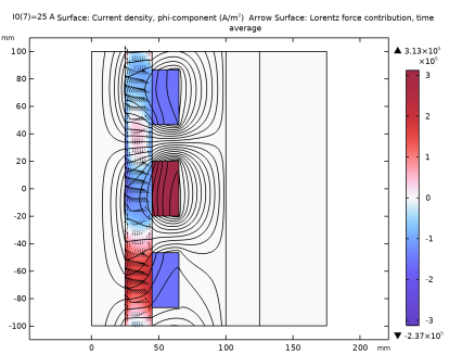
In the Settings window for Surface, click Replace Expression in the upper-right corner of the Expression section. From the menu, choose Component 1 (comp1) > Magnetic Fields > Currents and charge > Current density - A/m² > mf.Jphi - Current density, phi-component.
|
|
3
|
|
4
|
|
5
|
|
1
|
|
1
|
|
2
|
|
3
|
|
1
|
|
2
|
In the Settings window for 2D Plot Group, type Lorentz Force and Current Density in the Label text field.
|
|
3
|
|
1
|
|
2
|
In the Settings window for Surface, click Replace Expression in the upper-right corner of the Expression section. From the menu, choose Component 1 (comp1) > Magnetic Fields > Currents and charge > Current density - A/m² > mf.Jphi - Current density, phi-component.
|
|
3
|
|
4
|
|
1
|
|
2
|
|
3
|
|
4
|
|
5
|
|
6
|
|
7
|
Clear the Color legend checkbox.
|
|
8
|
|
1
|
|
2
|
In the Settings window for Arrow Surface, click Replace Expression in the upper-right corner of the Expression section. From the menu, choose Component 1 (comp1) > Magnetic Fields > Mechanical > mf.FLtzavr,mf.FLtzavz - Lorentz force contribution, time average.
|
|
3
|
Locate the Arrow Positioning section. Find the R grid points subsection. From the Entry method list, choose Coordinates.
|
|
4
|
|
5
|
|
6
|
|
7
|
|
1
|
|
2
|
|
3
|
|
4
|
|
1
|
|
2
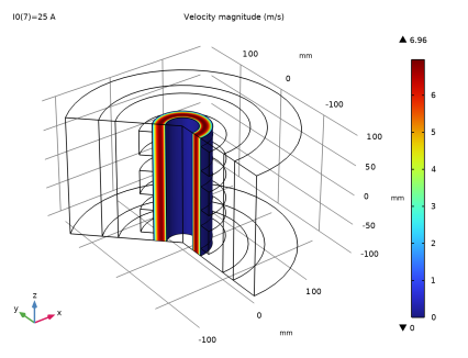
|
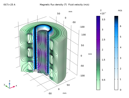
In the Settings window for 3D Plot Group, type Velocity and Magnetic Flux Density, Revolved Geometry in the Label text field.
|
|
3
|
|
4
|
|
1
|
|
2
|
|
3
|
|
4
|
|
5
|
|
6
|
Locate the Expression section.
|
|
7
|
|
8
|
|
1
|
In the Model Builder window, right-click Velocity and Magnetic Flux Density, Revolved Geometry and choose Volume.
|
|
2
|
|
3
|
|
4
|
|
5
|
|
6
|
|
7
|
|
8
|
|
1
|
|
2
|
|
3
|
|
4
|
|
5
|
|
6
|
Locate the Scale section.
|
|
7
|
|
1
|
In the Model Builder window, right-click Velocity and Magnetic Flux Density, Revolved Geometry and choose Contour.
|
|
2
|
|
3
|
|
4
|
|
5
|
|
6
|
|
7
|
Clear the Color legend checkbox.
|
|
8
|
|
1
|
|
2
|
|
3
|