PDF

Magnetic Signature of a Submarine
Introduction
A vessel traveling on the surface or under water gives rise to detectable local disturbances in Earth’s magnetic field. These disturbances can be used to trigger weapon systems. The magnetic signature of a ship can be reduced by generating a counteracting magnetic field of suitable strength and direction based on prior knowledge of the magnetic properties of the vessel. An important step in the design of a naval ship is therefore to predict its magnetic signature. Another application where magnetic signatures are of great importance is in urban traffic control: magnetic sensors, buried in our streets, are used to sense vehicles and control traffic lights.
Ships and cars are both to a large extent made of sheet metal. This makes them hard to simulate using standard finite element analysis because volume meshes of thin extended structures are difficult to generate and tend to become very large. This application demonstrates a powerful technique that circumvents the problem by modeling the sheet metal as 2D faces embedded in a 3D geometry. Thus it is only necessary to create comparatively inexpensive 2D face meshes in addition to the 3D volume mesh used for the surrounding medium. A tangential projection of the 3D equation is then solved on the 2D face mesh.
Figure 1: Submarine HMAS Collins. Image courtesy of Kockums AB.
This application also demonstrates the use of the reduced field formulation available in the AC/DC Module. This feature provides a convenient way to obtain the magnetic signature of the submarine by allowing the user to define the background field as a predefined quantity and solving only for the perturbations in this field.
Model Definition
In magnetostatic problems, where no currents are present, the problem can be solved using a scalar magnetic potential. This application demonstrates a special technique for modeling thin sheets of high-permeability materials and also shows the use of the reduced field formulation in the AC/DC Module for conveniently modeling perturbations in a known background field.
The model geometry is shown in Figure 2 and consists of face objects representing the submarine. The submarine geometry is based on the BeTSSi (Benchmark Target Echo Strength Simulation) benchmark submarine, as shown in Ref. 1 and Ref. 2, and does not represent a specific submarine class. A 3D box representing the surrounding water encloses the vessel (not shown).
Figure 2: The model geometry based on the BeTSSi submarine geometry.
Domain Equations
In a current-free region, where
it is possible to define the scalar magnetic potential, Vm, from the relation
This is analogous to the definition of the electric potential for static electric fields. Using the constitutive relation between the magnetic flux density and magnetic field
together with the equation
an equation for Vm can be derived,
In this model, you use the reduced field formulation, which means that you only solve for the potential Vm corresponding to the perturbation (reduced) field, so the equation you solve reads as
where Bext is a known background field, in this case, Earth’s magnetic field of 0.5 G.
Boundary Conditions
The exterior boundaries of the box are insulating for the reduced magnetic field:
On the face objects representing the hull of the submarine, you apply a 2D tangential projection of the 3D domain equation where the thickness and permeability of the hull are introduced as parameters. This is readily available in the used formulation as a shielding boundary condition, which is useful for modeling highly permeable thin sheets. Corresponding boundary conditions are available in the Electric Currents and Electrostatics interfaces for modeling of thin sheets with high conductance and high permittivity, respectively.
Results and Discussion
Figure 3 shows the total magnetic flux density in a horizontal slice plot 30 m below the submarine. A distinct field perturbation due to the presence of the vessel can be seen. The magnitude of the tangential magnetic field on the hull of the vessel is shown using contour lines. The reduced field is visualized as a streamline of the reduced magnetic potential surrounding the submarine. This gives a good picture of the perturbation caused by the presence of the submarine in the background field.
Figure 3: The slice color plot shows the total magnetic flux density (right color legend, uT). The contours on the submarine show the strength of the tangential magnetic field in the hull (left color legend, mT). The red streamlines show the reduced magnetic field.
Notes About the COMSOL Implementation
The model uses an MPHBIN-file as the starting geometry. It is possible to generate this geometry using COMSOL functionality. The instructions to do so are covered in the Appendix — Geometry Modeling Instructions. Due to the complexity of the geometry and the use of Cap Face operations, the generation of the geometry requires the CAD Import Module and the Design Module. The steps and operations for building the geometry include some geometry information like parameters, coordinates, and curve parameterizations, found in Appendix C of Ref. 2. The steps for building the geometry, using the COMSOL Geometry operations, do differ in some aspects from those in Ref. 2.
References
1. B. Nolte, I. Schäfer, C. de Jong, and L. Gilroy, “BeTSSi II benchmark on target strength simulation,” Proceedings of Forum Acusticum, 2014.
2. J.V. Venås and T. Kvamsdal, “Isogeometric boundary element method for acoustic scattering by a submarine,” Comp. Meth. Appl. Mech. Eng., vol. 359, p. 112670, 2020, doi.org/10.1016/j.cma.2019.112670.
Application Library path: ACDC_Module/Introductory_Magnetostatics/magnetic_signature_submarine
Modeling Instructions
From the File menu, choose New.
New
In the New window, click  Model Wizard.
Model Wizard
1
In the Model Wizard window, click  3D.
2
In the Select Physics tree, select AC/DC > Magnetic Fields, No Currents > Magnetic Fields, No Currents (mfnc).
3
Click Add.
4
Click  Study.
5
In the Select Study tree, select General Studies > Stationary.
6
Global Definitions
Define a parameter for the strength of the geomagnetic field and the dimensions of the water domain surrounding the submarine.
Parameters 1
1
In the Model Builder window, under Global Definitions click Parameters 1.
2
In the Settings window for Parameters, locate the Parameters section.
3
Geometry 1
The model uses an external geometry file with the submarine geometry added to a water domain.
Block 1 (blk1)
1
In the Geometry toolbar, click  Block.
2
In the Settings window for Block, locate the Size and Shape section.
3
In the Width text field, type dl.
4
In the Depth text field, type dw.
5
In the Height text field, type dw.
6
Locate the Position section. From the Base list, choose Center.
7
In the x text field, type dl/4.
8
In the Model Builder window, click Geometry 1.
9
In the Settings window for Geometry, locate the Cleanup section.
10
Clear the Automatic detection of small details checkbox.
Import 1 (imp1)
1
In the Home toolbar, click  Import.
2
In the Settings window for Import, locate the Source section.
3
Click  Browse.
4
5
Click  Import.
Definitions
Submarine
1
In the Definitions toolbar, click  Explicit.
For later use, define a boundary selection that corresponds to the submarine hull.
2
In the Settings window for Explicit, locate the Output Entities section.
3
From the Output entities list, choose Adjacent boundaries.
4
5
In the Label text field, type Submarine.
Geometry 1
Form Union (fin)
1
In the Geometry toolbar, click  Build All.
2
Click the  Go to Default View button in the Graphics toolbar.
3
Click the  Wireframe Rendering button in the Graphics toolbar.
Materials
Domain Material
1
In the Materials toolbar, click  Blank Material.
2
In the Settings window for Material, type Domain Material in the Label text field.
3
Click to expand the Material Properties section. In the Material properties tree, select Basic Properties > Relative Permeability.
4
Click  Add to Material.
5
Locate the Material Contents section. In the table, enter the following settings:
Hull Metal
1
In the Model Builder window, right-click Materials and choose Blank Material.
2
In the Settings window for Material, type Hull Metal in the Label text field.
Select the boundary selection named as Submarine as defined earlier.
3
Locate the Geometric Entity Selection section. From the Geometric entity level list, choose Boundary.
4
From the Selection list, choose Submarine.
5
Locate the Material Properties section. In the Material properties tree, select Basic Properties > Relative Permeability.
6
Click  Add to Material.
7
Locate the Material Contents section. In the table, enter the following settings:
Magnetic Fields, No Currents (mfnc)
Apply a background magnetic field corresponding to Earth’s geomagnetic field.
1
In the Model Builder window, under Component 1 (comp1) click Magnetic Fields, No Currents (mfnc).
2
In the Settings window for Magnetic Fields, No Currents, locate the Background Magnetic Field section.
3
From the Solve for list, choose Reduced field.
4
Specify the Hb vector as
The External Magnetic Flux Density feature imposes boundary conditions matching the specified background field.
External Magnetic Flux Density 1
1
In the Physics toolbar, click  Boundaries and choose External Magnetic Flux Density.
2
In the Settings window for External Magnetic Flux Density, locate the Boundary Selection section.
3
From the Selection list, choose All boundaries.
Zero Magnetic Scalar Potential 1
1
In the Physics toolbar, click  Points and choose Zero Magnetic Scalar Potential.
2
The Magnetic Shielding feature models a thin layer of high-permeability material, such as the metal constituting the submarine hull.
Magnetic Shielding 1
1
In the Physics toolbar, click  Boundaries and choose Magnetic Shielding.
2
In the Settings window for Magnetic Shielding, locate the Boundary Selection section.
3
From the Selection list, choose Submarine.
4
Locate the Magnetic Shielding section. In the ds text field, type 0.05.
5
Click the  Wireframe Rendering button in the Graphics toolbar.
Hide the boundaries of the water domain to show only the submarine.
6
Click the  Click and Hide button in the Graphics toolbar.
7
In the Graphics window toolbar, clicknext to  Select Boundaries, then choose Select Boundaries.
8
9
Click the  Click and Hide button in the Graphics toolbar.
Mesh 1
The default mesh settings will adequately resolve the region around the submarine hull.
Information
1
In the Model Builder window, under Component 1 (comp1) right-click Mesh 1 and choose Build All.
2
Click the  Zoom Extents button in the Graphics toolbar.
Study 1
Disable the automatic generation of default plots. Instead, you will create a custom plot when the solver has finished.
1
In the Settings window for Study, locate the Study Settings section.
2
Clear the Generate default plots checkbox.
3
In the Study toolbar, click  Compute.
Results
3D Plot Group 1
1
In the Model Builder window, expand the Results node.
2
Right-click Results and choose 3D Plot Group.
3
In the Settings window for 3D Plot Group, locate the Color Legend section.
4
Select the Show units checkbox.
5
Locate the Plot Settings section. Clear the Plot dataset edges checkbox.
First, create a slice plot to visualize the magnetic signature of the submarine 30 m away.
Slice 1
1
Right-click 3D Plot Group 1 and choose Slice.
2
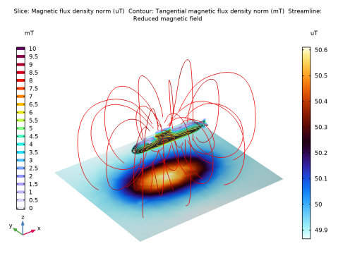
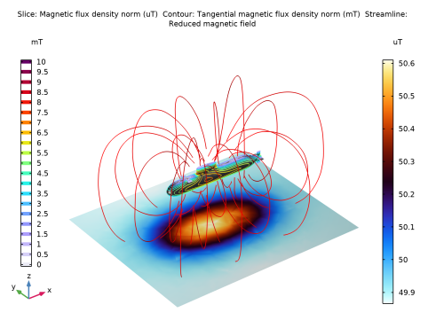
In the Settings window for Slice, click Replace Expression in the upper-right corner of the Expression section. From the menu, choose Component 1 (comp1) > Magnetic Fields, No Currents > Magnetic > mfnc.normB - Magnetic flux density norm - T.
3
Locate the Expression section. In the Unit field, type uT.
4
Locate the Plane Data section. From the Plane list, choose xy-planes.
5
From the Entry method list, choose Coordinates.
6
In the z-coordinates text field, type -30.
7
Locate the Coloring and Style section. From the Color table list, choose ThermalWaveDark.
8
In the 3D Plot Group 1 toolbar, click  Plot.
3D Plot Group 1
1
In the Model Builder window, click 3D Plot Group 1.
2
In the Settings window for 3D Plot Group, locate the Color Legend section.
3
From the Position list, choose Alternating.
The submarine can be represented by adding a material appearance to the surface.
Surface 1
1
Right-click 3D Plot Group 1 and choose Surface.
2
In the Settings window for Surface, locate the Expression section.
3
In the Expression text field, type 1.
Selection 1
1
Right-click Surface 1 and choose Selection.
2
In the Settings window for Selection, locate the Selection section.
3
From the Selection list, choose Submarine.
Surface 1
1
In the Model Builder window, click Surface 1.
2
In the Settings window for Surface, click to expand the Title section.
3
From the Title type list, choose None.
Material Appearance 1
1
Right-click Surface 1 and choose Material Appearance.
2
In the Settings window for Material Appearance, locate the Appearance section.
3
From the Appearance list, choose Custom.
4
From the Material type list, choose Iron (scratched).
3D Plot Group 1
Next, plot the tangential magnetic flux density across the hull of the submarine.
Contour 1
1
In the Model Builder window, right-click 3D Plot Group 1 and choose Contour.
2
In the Settings window for Contour, click Replace Expression in the upper-right corner of the Expression section. From the menu, choose Component 1 (comp1) > Magnetic Fields, No Currents > Magnetic > mfnc.normtB - Tangential magnetic flux density norm - T.
3
Locate the Levels section. From the Entry method list, choose Levels.
4
In the Levels text field, type range(0,0.5,10).
5
Locate the Expression section. From the Unit list, choose mT.
6
Locate the Coloring and Style section. From the Color table list, choose Prism.
3D Plot Group 1
In the Model Builder window, click 3D Plot Group 1.
Streamline 1
1
In the 3D Plot Group 1 toolbar, click  Streamline.
2
In the Settings window for Streamline, click Replace Expression in the upper-right corner of the Expression section. From the menu, choose Component 1 (comp1) > Magnetic Fields, No Currents > Magnetic > mfnc.redHx,...,mfnc.redHz - Reduced magnetic field.
3
Locate the Streamline Positioning section. From the Positioning list, choose Magnitude controlled.
4
Click the  Show Grid button in the Graphics toolbar.
5
In the 3D Plot Group 1 toolbar, click  Plot.
6
Click the  Zoom Extents button in the Graphics toolbar.
To visualize the perturbation of the background magnetic field, we can plot the scalar magnetic potential using the previous plot as a starting point.
3D Plot Group 2
1
Right-click 3D Plot Group 1 and choose Duplicate.
2
Click the  Go to XZ View button in the Graphics toolbar.
3
Click the  Orthographic Projection button in the Graphics toolbar.
Slice 1
1
In the Model Builder window, expand the 3D Plot Group 2 node, then click Slice 1.
2
In the Settings window for Slice, locate the Expression section.
3
In the Expression text field, type Vm.
4
Locate the Plane Data section. From the Plane list, choose zx-planes.
5
In the Planes text field, type 1.
6
Locate the Coloring and Style section. From the Scale list, choose Linear symmetric.
Streamline 1
1
In the Model Builder window, right-click Streamline 1 and choose Disable.
2
In the 3D Plot Group 2 toolbar, click  Plot.
The plot shows the effect of the submarine’s hull on the geomagnetic field.
Appendix — Geometry Modeling Instructions
From the File menu, choose New.
New
In the New window, click  Model Wizard.
Model Wizard
1
In the Model Wizard window, click  3D.
2
Geometry 1
1
In the Model Builder window, under Component 1 (comp1) click Geometry 1.
2
In the Settings window for Geometry, locate the Advanced section.
3
From the Geometry representation list, choose CAD kernel.
Disable the analysis of the geometry as the remaining small geometric details can be kept.
4
Locate the Cleanup section. Clear the Automatic detection of small details checkbox.
Global Definitions
Geometry Parameters
1
In the Model Builder window, under Global Definitions click Parameters 1.
2
In the Settings window for Parameters, locate the Parameters section.
3
Click  Load from File.
4
Browse to the model’s Application Libraries folder and double-click the file magnetic_signature_submarine_geom_sequence_parameters.txt.
5
In the Label text field, type Geometry Parameters.
Geometry 1
Work Plane 1 (wp1)
In the Geometry toolbar, click  Work Plane.
Work Plane 1 (wp1) > Plane Geometry
In the Model Builder window, click Plane Geometry.
Work Plane 1 (wp1) > Ellipse 1 (e1)
1
In the Work Plane toolbar, click  Ellipse.
2
In the Settings window for Ellipse, locate the Object Type section.
3
From the Type list, choose Curve.
4
Locate the Size and Shape section. In the a-semiaxis text field, type b.
5
In the b-semiaxis text field, type a.
6
In the Sector angle text field, type 90.
7
Locate the Position section. In the xw text field, type a.
8
Locate the Rotation Angle section. In the Rotation text field, type 90.
9
Click  Build Selected.
Work Plane 1 (wp1) > Line Segment 1 (ls1)
1
In the Work Plane toolbar, click  More Primitives and choose Line Segment.
2
On the object e1, select Point 1 only.
3
In the Settings window for Line Segment, locate the Endpoint section.
4
From the Specify list, choose Coordinates.
5
In the xw text field, type a+L.
6
In the yw text field, type b.
7
Click  Build Selected.
8
Click the  Zoom Extents button in the Graphics toolbar.
Work Plane 1 (wp1) > Circle 1 (c1)
1
In the Work Plane toolbar, click  Circle.
2
In the Settings window for Circle, locate the Object Type section.
3
From the Type list, choose Curve.
4
Locate the Size and Shape section. In the Radius text field, type g2/sin(alpha).
5
In the Sector angle text field, type alpha.
6
Locate the Position section. In the xw text field, type a+L.
7
In the yw text field, type b-g2/sin(alpha).
8
Locate the Rotation Angle section. In the Rotation text field, type 90-alpha.
9
Click  Build Selected.
Work Plane 1 (wp1) > Line Segment 2 (ls2)
1
In the Work Plane toolbar, click  More Primitives and choose Line Segment.
2
On the object c1, select Point 1 only.
3
In the Settings window for Line Segment, locate the Endpoint section.
4
From the Specify list, choose Coordinates.
5
In the xw text field, type a+L+g2+g3.
6
In the yw text field, type (b-(1-cos(alpha))*g2/sin(alpha))-g3*tan(alpha).
7
Click  Build Selected.
8
Click the  Zoom Extents button in the Graphics toolbar.
Work Plane 1 (wp1) > Delete Entities 1 (del1)
1
Right-click Plane Geometry and choose Delete Entities.
2
On the object c1, select Boundaries 2 and 3 only.
3
On the object e1, select Boundaries 2 and 3 only.
4
In the Work Plane toolbar, click  Build All.
Revolve 1 (rev1)
1
In the Model Builder window, under Component 1 (comp1) > Geometry 1 right-click Work Plane 1 (wp1) and choose Revolve.
2
In the Settings window for Revolve, locate the Revolution Angles section.
3
Click the Angles button.
4
In the Start angle text field, type 60[deg].
5
In the End angle text field, type 180[deg].
6
Locate the Revolution Axis section. Find the Direction of revolution axis subsection. In the xw text field, type 1.
7
In the yw text field, type 0.
8
Click  Build Selected.
Work Plane 2 (wp2)
1
In the Geometry toolbar, click  Work Plane.
2
In the Settings window for Work Plane, locate the Plane Definition section.
3
From the Plane list, choose zy-plane.
4
In the x-coordinate text field, type a.
5
Click  Build Selected.
Work Plane 2 (wp2) > Plane Geometry
In the Model Builder window, click Plane Geometry.
Work Plane 2 (wp2) > Polygon 1 (pol1)
1
In the Work Plane toolbar, click  Polygon.
2
In the Settings window for Polygon, locate the Object Type section.
3
From the Type list, choose Open curve.
4
Locate the Coordinates section. In the table, enter the following settings:
5
Click  Build Selected.
6
Click the  Zoom Extents button in the Graphics toolbar.
Extrude 1 (ext1)
1
In the Model Builder window, under Component 1 (comp1) > Geometry 1 right-click Work Plane 2 (wp2) and choose Extrude.
2
In the Settings window for Extrude, locate the Distances section.
3
4
Select the Reverse direction checkbox.
5
Click  Build Selected.
Work Plane 3 (wp3)
1
In the Geometry toolbar, click  Work Plane.
2
In the Settings window for Work Plane, locate the Plane Definition section.
3
From the Plane type list, choose Coordinates.
4
In row Point 3, set y to cos(theta).
5
In row Point 3, set z to sin(theta).
Work Plane 3 (wp3) > Plane Geometry
In the Model Builder window, click Plane Geometry.
Work Plane 3 (wp3) > Line Segment 1 (ls1)
1
In the Work Plane toolbar, click  More Primitives and choose Line Segment.
2
In the Settings window for Line Segment, locate the Starting Point section.
3
From the Specify list, choose Coordinates.
4
In the xw text field, type a+L+g2.
5
In the yw text field, type (b-(1-cos(alpha))*g2/sin(alpha)).
6
Locate the Endpoint section. From the Specify list, choose Coordinates.
7
In the xw text field, type a+L+g2+g3.
8
In the yw text field, type (b-(1-cos(alpha))*g2/sin(alpha))-g3*tan(alpha).
9
Click  Build Selected.
Revolve 2 (rev2)
1
In the Model Builder window, under Component 1 (comp1) > Geometry 1 right-click Work Plane 3 (wp3) and choose Revolve.
2
In the Settings window for Revolve, locate the Revolution Angles section.
3
Click the Angles button.
4
In the End angle text field, type -60.
5
Locate the Revolution Axis section. Find the Direction of revolution axis subsection. In the xw text field, type 1.
6
In the yw text field, type 0.
7
Click  Build Selected.
Work Plane 4 (wp4)
1
In the Geometry toolbar, click  Work Plane.
2
In the Settings window for Work Plane, locate the Plane Definition section.
3
From the Plane type list, choose Coordinates.
4
In row Point 3, set x to 7.
5
In row Point 3, set y to c_deck.
6
In row Point 3, set z to s_deck.
7
Click  Build Selected.
Work Plane 4 (wp4) > Plane Geometry
In the Model Builder window, click Plane Geometry.
Work Plane 4 (wp4) > Ellipse 1 (e1)
1
In the Work Plane toolbar, click  Ellipse.
2
In the Settings window for Ellipse, locate the Object Type section.
3
From the Type list, choose Curve.
4
Locate the Size and Shape section. In the a-semiaxis text field, type a.
5
In the b-semiaxis text field, type sqrt(c_deck^2+s_deck^2).
6
In the Sector angle text field, type 180.
7
Locate the Position section. In the xw text field, type a.
8
Click  Build Selected.
Work Plane 4 (wp4) > Interpolation Curve 1 (ic1)
1
In the Work Plane toolbar, click  More Primitives and choose Interpolation Curve.
2
In the Settings window for Interpolation Curve, locate the Interpolation Points section.
3
4
Click  Build Selected.
Work Plane 4 (wp4) > Line Segment 1 (ls1)
1
In the Work Plane toolbar, click  More Primitives and choose Line Segment.
2
In the Settings window for Line Segment, locate the Starting Point section.
3
From the Specify list, choose Coordinates.
4
In the xw text field, type a+L.
5
Locate the Endpoint section. From the Specify list, choose Coordinates.
6
In the xw text field, type a+L.
7
In the yw text field, type c_deck+s_deck.
8
Click  Build Selected.
Work Plane 4 (wp4) > Line Segment 2 (ls2)
1
In the Work Plane toolbar, click  More Primitives and choose Line Segment.
2
In the Settings window for Line Segment, locate the Starting Point section.
3
From the Specify list, choose Coordinates.
4
In the xw text field, type a+L+g2.
5
Locate the Endpoint section. From the Specify list, choose Coordinates.
6
In the xw text field, type a+L+g2.
7
In the yw text field, type c_deck+s_deck.
8
Click  Build Selected.
Work Plane 4 (wp4) > Union 1 (uni1)
1
In the Work Plane toolbar, click  Booleans and Partitions and choose Union.
2
Click the  Select All button in the Graphics toolbar.
3
In the Settings window for Union, click  Build Selected.
Work Plane 4 (wp4) > Delete Entities 1 (del1)
1
Right-click Plane Geometry and choose Delete Entities.
2
On the object uni1, select Boundaries 1–6, 8, 9, and 11 only.
3
In the Settings window for Delete Entities, click  Build Selected.
Work Plane 4 (wp4)
1
In the Model Builder window, under Component 1 (comp1) > Geometry 1 click Work Plane 4 (wp4).
2
In the Settings window for Work Plane, click  Build Selected.
Work Plane 5 (wp5)
1
In the Geometry toolbar, click  Work Plane.
2
In the Settings window for Work Plane, locate the Plane Definition section.
3
From the Plane type list, choose Coordinates.
4
In row Point 3, set x to 7.
5
In row Point 3, set y to c_deck-(p_a*((-sin(theta)*b+s_deck)/6)^3+p_b*((-sin(theta)*b+s_deck)/6)^2).
6
In row Point 3, set z to -(-sin(theta)*b+s_deck)/6+s_deck.
7
Click  Build Selected.
Work Plane 5 (wp5) > Plane Geometry
In the Model Builder window, click Plane Geometry.
Work Plane 5 (wp5) > Ellipse 1 (e1)
1
In the Work Plane toolbar, click  Ellipse.
2
In the Settings window for Ellipse, locate the Object Type section.
3
From the Type list, choose Curve.
4
Locate the Size and Shape section. In the a-semiaxis text field, type a.
5
In the b-semiaxis text field, type sqrt((c_deck-(p_a*((-sin(theta)*b+s_deck)/6)^3+p_b*((-sin(theta)*b+s_deck)/6)^2))^2+(-(-sin(theta)*b+s_deck)/6+s_deck)^2).
6
In the Sector angle text field, type 180.
7
Locate the Position section. In the xw text field, type a.
8
Click  Build Selected.
Work Plane 5 (wp5) > Interpolation Curve 1 (ic1)
1
In the Work Plane toolbar, click  More Primitives and choose Interpolation Curve.
2
In the Settings window for Interpolation Curve, locate the Interpolation Points section.
3
4
Click  Build Selected.
Work Plane 5 (wp5) > Line Segment 1 (ls1)
1
In the Work Plane toolbar, click  More Primitives and choose Line Segment.
2
In the Settings window for Line Segment, locate the Starting Point section.
3
From the Specify list, choose Coordinates.
4
In the xw text field, type a+L.
5
Locate the Endpoint section. From the Specify list, choose Coordinates.
6
In the xw text field, type a+L.
7
In the yw text field, type c_deck+s_deck.
8
Click  Build Selected.
Work Plane 5 (wp5) > Line Segment 2 (ls2)
1
In the Work Plane toolbar, click  More Primitives and choose Line Segment.
2
In the Settings window for Line Segment, locate the Starting Point section.
3
From the Specify list, choose Coordinates.
4
In the xw text field, type a+L+g2.
5
Locate the Endpoint section. From the Specify list, choose Coordinates.
6
In the xw text field, type a+L+g2.
7
In the yw text field, type c_deck+s_deck.
8
Click  Build Selected.
Work Plane 5 (wp5) > Union 1 (uni1)
1
In the Work Plane toolbar, click  Booleans and Partitions and choose Union.
2
Click the  Select All button in the Graphics toolbar.
3
In the Settings window for Union, click  Build Selected.
Work Plane 5 (wp5) > Delete Entities 1 (del1)
1
Right-click Plane Geometry and choose Delete Entities.
2
On the object uni1, select Boundaries 1–6, 8, 9, and 11 only.
3
In the Settings window for Delete Entities, click  Build Selected.
Work Plane 5 (wp5)
1
In the Model Builder window, under Component 1 (comp1) > Geometry 1 click Work Plane 5 (wp5).
2
In the Settings window for Work Plane, click  Build Selected.
Work Plane 6 (wp6)
1
In the Geometry toolbar, click  Work Plane.
2
In the Settings window for Work Plane, locate the Plane Definition section.
3
From the Plane type list, choose Coordinates.
4
In row Point 3, set x to 7.
5
In row Point 3, set y to c_deck-(p_a*((-sin(theta)*b+s_deck)*2/6)^3+p_b*((-sin(theta)*b+s_deck)*2/6)^2).
6
In row Point 3, set z to -(-sin(theta)*b+s_deck)*2/6+s_deck.
7
Click  Build Selected.
Work Plane 6 (wp6) > Plane Geometry
In the Model Builder window, click Plane Geometry.
Work Plane 6 (wp6) > Ellipse 1 (e1)
1
In the Work Plane toolbar, click  Ellipse.
2
In the Settings window for Ellipse, locate the Object Type section.
3
From the Type list, choose Curve.
4
Locate the Size and Shape section. In the a-semiaxis text field, type a.
5
In the b-semiaxis text field, type sqrt((c_deck-(p_a*((-sin(theta)*b+s_deck)*2/6)^3+p_b*((-sin(theta)*b+s_deck)*2/6)^2))^2+(-(-sin(theta)*b+s_deck)*2/6+s_deck)^2).
6
In the Sector angle text field, type 180.
7
Locate the Position section. In the xw text field, type a.
8
Click  Build Selected.
Work Plane 6 (wp6) > Interpolation Curve 1 (ic1)
1
In the Work Plane toolbar, click  More Primitives and choose Interpolation Curve.
2
In the Settings window for Interpolation Curve, locate the Interpolation Points section.
3
4
Click  Build Selected.
Work Plane 6 (wp6) > Line Segment 1 (ls1)
1
In the Work Plane toolbar, click  More Primitives and choose Line Segment.
2
In the Settings window for Line Segment, locate the Starting Point section.
3
From the Specify list, choose Coordinates.
4
In the xw text field, type a+L.
5
Locate the Endpoint section. From the Specify list, choose Coordinates.
6
In the xw text field, type a+L.
7
In the yw text field, type c_deck+s_deck.
8
Click  Build Selected.
Work Plane 6 (wp6) > Line Segment 2 (ls2)
1
In the Work Plane toolbar, click  More Primitives and choose Line Segment.
2
In the Settings window for Line Segment, locate the Starting Point section.
3
From the Specify list, choose Coordinates.
4
In the xw text field, type a+L+g2.
5
Locate the Endpoint section. From the Specify list, choose Coordinates.
6
In the xw text field, type a+L+g2.
7
In the yw text field, type c_deck+s_deck.
8
Click  Build Selected.
Work Plane 6 (wp6) > Union 1 (uni1)
1
In the Work Plane toolbar, click  Booleans and Partitions and choose Union.
2
Click the  Select All button in the Graphics toolbar.
3
In the Settings window for Union, click  Build Selected.
Work Plane 6 (wp6) > Delete Entities 1 (del1)
1
Right-click Plane Geometry and choose Delete Entities.
2
On the object uni1, select Boundaries 1–6, 8, 9, and 11 only.
3
In the Settings window for Delete Entities, click  Build Selected.
Work Plane 6 (wp6)
1
In the Model Builder window, under Component 1 (comp1) > Geometry 1 click Work Plane 6 (wp6).
2
In the Settings window for Work Plane, click  Build Selected.
Work Plane 7 (wp7)
1
In the Geometry toolbar, click  Work Plane.
2
In the Settings window for Work Plane, locate the Plane Definition section.
3
From the Plane type list, choose Coordinates.
4
In row Point 3, set x to 7.
5
In row Point 3, set y to c_deck-(p_a*((-sin(theta)*b+s_deck)*3/6)^3+p_b*((-sin(theta)*b+s_deck)*3/6)^2).
6
In row Point 3, set z to -(-sin(theta)*b+s_deck)*3/6+s_deck.
7
Click  Build Selected.
Work Plane 7 (wp7) > Plane Geometry
In the Model Builder window, click Plane Geometry.
Work Plane 7 (wp7) > Ellipse 1 (e1)
1
In the Work Plane toolbar, click  Ellipse.
2
In the Settings window for Ellipse, locate the Object Type section.
3
From the Type list, choose Curve.
4
Locate the Size and Shape section. In the a-semiaxis text field, type a.
5
In the b-semiaxis text field, type sqrt((c_deck-(p_a*((-sin(theta)*b+s_deck)*3/6)^3+p_b*((-sin(theta)*b+s_deck)*3/6)^2))^2+(-(-sin(theta)*b+s_deck)*3/6+s_deck)^2).
6
In the Sector angle text field, type 180.
7
Locate the Position section. In the xw text field, type a.
8
Click  Build Selected.
Work Plane 7 (wp7) > Interpolation Curve 1 (ic1)
1
In the Work Plane toolbar, click  More Primitives and choose Interpolation Curve.
2
In the Settings window for Interpolation Curve, locate the Interpolation Points section.
3
4
Click  Build Selected.
Work Plane 7 (wp7) > Line Segment 1 (ls1)
1
In the Work Plane toolbar, click  More Primitives and choose Line Segment.
2
In the Settings window for Line Segment, locate the Starting Point section.
3
From the Specify list, choose Coordinates.
4
In the xw text field, type a+L.
5
Locate the Endpoint section. From the Specify list, choose Coordinates.
6
In the xw text field, type a+L.
7
In the yw text field, type c_deck+s_deck.
8
Click  Build Selected.
Work Plane 7 (wp7) > Line Segment 2 (ls2)
1
In the Work Plane toolbar, click  More Primitives and choose Line Segment.
2
In the Settings window for Line Segment, locate the Starting Point section.
3
From the Specify list, choose Coordinates.
4
In the xw text field, type a+L+g2.
5
Locate the Endpoint section. From the Specify list, choose Coordinates.
6
In the xw text field, type a+L+g2.
7
In the yw text field, type c_deck+s_deck.
8
Click  Build Selected.
Work Plane 7 (wp7) > Union 1 (uni1)
1
In the Work Plane toolbar, click  Booleans and Partitions and choose Union.
2
Click the  Select All button in the Graphics toolbar.
3
In the Settings window for Union, click  Build Selected.
Work Plane 7 (wp7) > Delete Entities 1 (del1)
1
Right-click Plane Geometry and choose Delete Entities.
2
On the object uni1, select Boundaries 1–6, 8, 9, and 11 only.
3
In the Settings window for Delete Entities, click  Build Selected.
Work Plane 7 (wp7)
1
In the Model Builder window, under Component 1 (comp1) > Geometry 1 click Work Plane 7 (wp7).
2
In the Settings window for Work Plane, click  Build Selected.
Work Plane 8 (wp8)
1
In the Geometry toolbar, click  Work Plane.
2
In the Settings window for Work Plane, locate the Plane Definition section.
3
From the Plane type list, choose Coordinates.
4
In row Point 3, set x to 7.
5
In row Point 3, set y to c_deck-(p_a*((-sin(theta)*b+s_deck)*4/6)^3+p_b*((-sin(theta)*b+s_deck)*4/6)^2).
6
In row Point 3, set z to -(-sin(theta)*b+s_deck)*4/6+s_deck.
7
Click  Build Selected.
Work Plane 8 (wp8) > Plane Geometry
In the Model Builder window, click Plane Geometry.
Work Plane 8 (wp8) > Ellipse 1 (e1)
1
In the Work Plane toolbar, click  Ellipse.
2
In the Settings window for Ellipse, locate the Object Type section.
3
From the Type list, choose Curve.
4
Locate the Size and Shape section. In the a-semiaxis text field, type a.
5
In the b-semiaxis text field, type sqrt((c_deck-(p_a*((-sin(theta)*b+s_deck)*4/6)^3+p_b*((-sin(theta)*b+s_deck)*4/6)^2))^2+(-(-sin(theta)*b+s_deck)*4/6+s_deck)^2).
6
In the Sector angle text field, type 180.
7
Locate the Position section. In the xw text field, type a.
8
Click  Build Selected.
Work Plane 8 (wp8) > Interpolation Curve 1 (ic1)
1
In the Work Plane toolbar, click  More Primitives and choose Interpolation Curve.
2
In the Settings window for Interpolation Curve, locate the Interpolation Points section.
3
4
Click  Build Selected.
Work Plane 8 (wp8) > Line Segment 1 (ls1)
1
In the Work Plane toolbar, click  More Primitives and choose Line Segment.
2
In the Settings window for Line Segment, locate the Starting Point section.
3
From the Specify list, choose Coordinates.
4
In the xw text field, type a+L.
5
Locate the Endpoint section. From the Specify list, choose Coordinates.
6
In the xw text field, type a+L.
7
In the yw text field, type c_deck+s_deck.
8
Click  Build Selected.
Work Plane 8 (wp8) > Line Segment 2 (ls2)
1
In the Work Plane toolbar, click  More Primitives and choose Line Segment.
2
In the Settings window for Line Segment, locate the Starting Point section.
3
From the Specify list, choose Coordinates.
4
In the xw text field, type a+L+g2.
5
Locate the Endpoint section. From the Specify list, choose Coordinates.
6
In the xw text field, type a+L+g2.
7
In the yw text field, type c_deck+s_deck.
8
Click  Build Selected.
Work Plane 8 (wp8) > Union 1 (uni1)
1
In the Work Plane toolbar, click  Booleans and Partitions and choose Union.
2
Click the  Select All button in the Graphics toolbar.
3
In the Settings window for Union, click  Build Selected.
Work Plane 8 (wp8) > Delete Entities 1 (del1)
1
Right-click Plane Geometry and choose Delete Entities.
2
On the object uni1, select Boundaries 1–6, 8, 9, and 11 only.
3
In the Settings window for Delete Entities, click  Build Selected.
Work Plane 8 (wp8)
1
In the Model Builder window, under Component 1 (comp1) > Geometry 1 click Work Plane 8 (wp8).
2
In the Settings window for Work Plane, click  Build Selected.
Work Plane 9 (wp9)
1
In the Geometry toolbar, click  Work Plane.
2
In the Settings window for Work Plane, locate the Plane Definition section.
3
From the Plane type list, choose Coordinates.
4
In row Point 3, set x to 7.
5
In row Point 3, set y to c_deck-(p_a*((-sin(theta)*b+s_deck)*5/6)^3+p_b*((-sin(theta)*b+s_deck)*5/6)^2).
6
In row Point 3, set z to -(-sin(theta)*b+s_deck)*5/6+s_deck.
7
Click  Build Selected.
Work Plane 9 (wp9) > Plane Geometry
In the Model Builder window, click Plane Geometry.
Work Plane 9 (wp9) > Ellipse 1 (e1)
1
In the Work Plane toolbar, click  Ellipse.
2
In the Settings window for Ellipse, locate the Object Type section.
3
From the Type list, choose Curve.
4
Locate the Size and Shape section. In the a-semiaxis text field, type a.
5
In the b-semiaxis text field, type sqrt((c_deck-(p_a*((-sin(theta)*b+s_deck)*5/6)^3+p_b*((-sin(theta)*b+s_deck)*5/6)^2))^2+(-(-sin(theta)*b+s_deck)*5/6+s_deck)^2).
6
In the Sector angle text field, type 180.
7
Locate the Position section. In the xw text field, type a.
8
Click  Build Selected.
Work Plane 9 (wp9) > Interpolation Curve 1 (ic1)
1
In the Work Plane toolbar, click  More Primitives and choose Interpolation Curve.
2
In the Settings window for Interpolation Curve, locate the Interpolation Points section.
3
4
Click  Build Selected.
Work Plane 9 (wp9) > Line Segment 1 (ls1)
1
In the Work Plane toolbar, click  More Primitives and choose Line Segment.
2
In the Settings window for Line Segment, locate the Starting Point section.
3
From the Specify list, choose Coordinates.
4
In the xw text field, type a+L.
5
Locate the Endpoint section. From the Specify list, choose Coordinates.
6
In the xw text field, type a+L.
7
In the yw text field, type c_deck+s_deck.
8
Click  Build Selected.
Work Plane 9 (wp9) > Line Segment 2 (ls2)
1
In the Work Plane toolbar, click  More Primitives and choose Line Segment.
2
In the Settings window for Line Segment, locate the Starting Point section.
3
From the Specify list, choose Coordinates.
4
In the xw text field, type a+L+g2.
5
Locate the Endpoint section. From the Specify list, choose Coordinates.
6
In the xw text field, type a+L+g2.
7
In the yw text field, type c_deck+s_deck.
8
Click  Build Selected.
Work Plane 9 (wp9) > Union 1 (uni1)
1
In the Work Plane toolbar, click  Booleans and Partitions and choose Union.
2
Click the  Select All button in the Graphics toolbar.
3
In the Settings window for Union, click  Build Selected.
Work Plane 9 (wp9) > Delete Entities 1 (del1)
1
Right-click Plane Geometry and choose Delete Entities.
2
On the object uni1, select Boundaries 1–6, 8, 9, and 11 only.
3
In the Settings window for Delete Entities, click  Build Selected.
Work Plane 9 (wp9)
1
In the Model Builder window, under Component 1 (comp1) > Geometry 1 click Work Plane 9 (wp9).
2
In the Settings window for Work Plane, click  Build Selected.
Work Plane 10 (wp10)
In the Geometry toolbar, click  Work Plane.
Work Plane 10 (wp10) > Plane Geometry
In the Model Builder window, click Plane Geometry.
Work Plane 10 (wp10) > Ellipse 1 (e1)
1
In the Work Plane toolbar, click  Ellipse.
2
In the Settings window for Ellipse, locate the Object Type section.
3
From the Type list, choose Curve.
4
Locate the Size and Shape section. In the a-semiaxis text field, type a.
5
In the b-semiaxis text field, type c_deck.
6
In the Sector angle text field, type 180.
7
Locate the Position section. In the xw text field, type a.
8
Click  Build Selected.
Work Plane 10 (wp10) > Interpolation Curve 1 (ic1)
1
In the Work Plane toolbar, click  More Primitives and choose Interpolation Curve.
2
In the Settings window for Interpolation Curve, locate the Interpolation Points section.
3
4
Click  Build Selected.
Work Plane 10 (wp10) > Line Segment 1 (ls1)
1
In the Work Plane toolbar, click  More Primitives and choose Line Segment.
2
In the Settings window for Line Segment, locate the Starting Point section.
3
From the Specify list, choose Coordinates.
4
In the xw text field, type a+L.
5
Locate the Endpoint section. From the Specify list, choose Coordinates.
6
In the xw text field, type a+L.
7
In the yw text field, type c_deck+s_deck.
8
Click  Build Selected.
Work Plane 10 (wp10) > Line Segment 2 (ls2)
1
In the Work Plane toolbar, click  More Primitives and choose Line Segment.
2
In the Settings window for Line Segment, locate the Starting Point section.
3
From the Specify list, choose Coordinates.
4
In the xw text field, type a+L+g2.
5
Locate the Endpoint section. From the Specify list, choose Coordinates.
6
In the xw text field, type a+L+g2.
7
In the yw text field, type c_deck+s_deck.
8
Click  Build Selected.
Work Plane 10 (wp10) > Union 1 (uni1)
1
In the Work Plane toolbar, click  Booleans and Partitions and choose Union.
2
Click the  Select All button in the Graphics toolbar.
3
In the Settings window for Union, click  Build Selected.
Work Plane 10 (wp10) > Delete Entities 1 (del1)
1
Right-click Plane Geometry and choose Delete Entities.
2
On the object uni1, select Boundaries 1–6, 8, 9, and 11 only.
3
In the Settings window for Delete Entities, click  Build Selected.
Work Plane 10 (wp10)
1
In the Model Builder window, under Component 1 (comp1) > Geometry 1 click Work Plane 10 (wp10).
2
In the Settings window for Work Plane, click  Build Selected.
Union 1 (uni1)
1
In the Geometry toolbar, click  Booleans and Partitions and choose Union.
2
Click the  Select All button in the Graphics toolbar.
3
In the Settings window for Union, click  Build Selected.
Cap Faces 1 (cap1)
1
In the Geometry toolbar, click  Defeaturing and Repair and choose Cap Faces.
2
On the object uni1, select Edges 46–48 and 60 only.
3
In the Settings window for Cap Faces, click  Build Selected.
Cap Faces 2 (cap2)
1
In the Geometry toolbar, click  Defeaturing and Repair and choose Cap Faces.
2
On the object cap1, select Edges 44, 45, 48, and 59 only.
3
In the Settings window for Cap Faces, click  Build Selected.
Cap Faces 3 (cap3)
1
In the Geometry toolbar, click  Defeaturing and Repair and choose Cap Faces.
2
On the object cap2, select Edges 42, 43, 45, and 58 only.
3
In the Settings window for Cap Faces, click  Build Selected.
Cap Faces 4 (cap4)
1
In the Geometry toolbar, click  Defeaturing and Repair and choose Cap Faces.
2
On the object cap3, select Edges 40, 41, 43, and 57 only.
3
In the Settings window for Cap Faces, click  Build Selected.
Cap Faces 5 (cap5)
1
In the Geometry toolbar, click  Defeaturing and Repair and choose Cap Faces.
2
On the object cap4, select Edges 38, 39, 41, and 56 only.
3
In the Settings window for Cap Faces, click  Build Selected.
Cap Faces 6 (cap6)
1
In the Geometry toolbar, click  Defeaturing and Repair and choose Cap Faces.
2
On the object cap5, select Edges 36, 37, 39, and 55 only.
3
In the Settings window for Cap Faces, click  Build Selected.
Cap Faces 7 (cap7)
1
In the Geometry toolbar, click  Defeaturing and Repair and choose Cap Faces.
2
On the object cap6, select Edges 34, 35, 37, and 53 only.
3
In the Settings window for Cap Faces, click  Build Selected.
Cap Faces 8 (cap8)
1
In the Geometry toolbar, click  Defeaturing and Repair and choose Cap Faces.
2
In the Settings window for Cap Faces, locate the Cap Faces section.
3
Click the  Clear Selection button for Bounding edges.
4
On the object cap7, select Edges 9, 10, and 27 only.
5
Click  Build Selected.
Cap Faces 9 (cap9)
1
In the Geometry toolbar, click  Defeaturing and Repair and choose Cap Faces.
2
On the object cap8, select Edges 8, 10, and 25 only.
3
In the Settings window for Cap Faces, click  Build Selected.
Cap Faces 10 (cap10)
1
In the Geometry toolbar, click  Defeaturing and Repair and choose Cap Faces.
2
On the object cap9, select Edges 7, 8, and 23 only.
3
In the Settings window for Cap Faces, click  Build Selected.
Cap Faces 11 (cap11)
1
In the Geometry toolbar, click  Defeaturing and Repair and choose Cap Faces.
2
On the object cap10, select Edges 6, 7, and 21 only.
3
In the Settings window for Cap Faces, click  Build Selected.
Cap Faces 12 (cap12)
1
In the Geometry toolbar, click  Defeaturing and Repair and choose Cap Faces.
2
On the object cap11, select Edges 5, 6, and 19 only.
3
In the Settings window for Cap Faces, click  Build Selected.
Cap Faces 13 (cap13)
1
In the Geometry toolbar, click  Defeaturing and Repair and choose Cap Faces.
2
On the object cap12, select Edges 4, 5, and 17 only.
3
In the Settings window for Cap Faces, click  Build Selected.
Cap Faces 14 (cap14)
1
In the Geometry toolbar, click  Defeaturing and Repair and choose Cap Faces.
2
On the object cap13, select Edges 3, 4, and 15 only.
3
In the Settings window for Cap Faces, click  Build Selected.
Work Plane 11 (wp11)
1
In the Geometry toolbar, click  Work Plane.
2
In the Settings window for Work Plane, locate the Plane Definition section.
3
From the Plane list, choose zx-plane.
4
In the y-coordinate text field, type c_deck.
5
Click to expand the Local Coordinate System section. In the Rotation text field, type 90.
6
Click  Build Selected.
Work Plane 11 (wp11) > Plane Geometry
In the Model Builder window, click Plane Geometry.
Work Plane 11 (wp11) > Parametric Curve 1 (pc1)
1
In the Work Plane toolbar, click  More Primitives and choose Parametric Curve.
2
In the Settings window for Parametric Curve, locate the Expressions section.
3
In the xw text field, type s_x1+s_l1*s.
4
In the yw text field, type -(5*2*s_deck/s_l1*(a0*s^0.5-a1*s-a2*s^2+a3*s^3-a4*s^4))*s_l1.
5
Locate the Advanced Settings section. Select the Reparameterize using arc length checkbox.
6
Click  Build Selected.
Work Plane 11 (wp11)
1
In the Model Builder window, under Component 1 (comp1) > Geometry 1 click Work Plane 11 (wp11).
2
In the Settings window for Work Plane, click  Build Selected.
Work Plane 12 (wp12)
1
In the Geometry toolbar, click  Work Plane.
2
In the Settings window for Work Plane, locate the Plane Definition section.
3
From the Plane list, choose zx-plane.
4
In the y-coordinate text field, type c_deck+s_h.
5
Locate the Local Coordinate System section. In the Rotation text field, type 90.
6
Click  Build Selected.
Work Plane 12 (wp12) > Plane Geometry
In the Model Builder window, click Plane Geometry.
Work Plane 12 (wp12) > Parametric Curve 1 (pc1)
1
In the Work Plane toolbar, click  More Primitives and choose Parametric Curve.
2
In the Settings window for Parametric Curve, locate the Expressions section.
3
In the xw text field, type s_x2+s_l2*s.
4
In the yw text field, type -(5*s_w2/s_l1*(a0*s^0.5-a1*s-a2*s^2+a3*s^3-a4*s^4))*s_l2.
5
Locate the Advanced Settings section. Select the Reparameterize using arc length checkbox.
6
Click  Build Selected.
Work Plane 12 (wp12) > Line Segment 1 (ls1)
1
In the Work Plane toolbar, click  More Primitives and choose Line Segment.
2
In the Settings window for Line Segment, locate the Starting Point section.
3
Click to select the  Activate Selection toggle button for Start vertex.
4
On the object pc1, select Point 1 only.
5
Locate the Endpoint section. Click to select the  Activate Selection toggle button for End vertex.
6
On the object pc1, select Point 2 only.
7
Click  Build Selected.
Work Plane 12 (wp12) > Convert to Solid 1 (csol1)
1
In the Work Plane toolbar, click  Conversions and choose Convert to Solid.
2
Click in the Graphics window and then press Ctrl+A to select both objects.
3
In the Settings window for Convert to Solid, click  Build Selected.
Work Plane 12 (wp12)
1
In the Model Builder window, under Component 1 (comp1) > Geometry 1 click Work Plane 12 (wp12).
2
In the Settings window for Work Plane, click  Build Selected.
Loft 1 (loft1)
1
In the Geometry toolbar, click  Loft.
2
In the Settings window for Loft, locate the General section.
3
Clear the Unite with input objects checkbox.
4
Click to expand the Start Profile section. From the Geometric entity level list, choose Edge.
5
On the object wp12, select Edge 2 only.
6
Click to expand the End Profile section. From the Geometric entity level list, choose Edge.
7
On the object wp11, select Edge 1 only.
8
Click  Build Selected.
Work Plane 13 (wp13)
1
In the Geometry toolbar, click  Work Plane.
2
In the Settings window for Work Plane, locate the Plane Definition section.
3
From the Plane list, choose yz-plane.
4
In the x-coordinate text field, type a+L+g2+g3.
Work Plane 13 (wp13) > Plane Geometry
In the Model Builder window, click Plane Geometry.
Work Plane 13 (wp13) > Circle 1 (c1)
1
In the Work Plane toolbar, click  Circle.
2
In the Settings window for Circle, locate the Size and Shape section.
3
In the Radius text field, type (b-(1-cos(alpha))*g2/sin(alpha))-g3*tan(alpha).
4
In the Sector angle text field, type 180.
5
Click  Build Selected.
Work Plane 13 (wp13)
1
In the Model Builder window, under Component 1 (comp1) > Geometry 1 click Work Plane 13 (wp13).
2
In the Settings window for Work Plane, click  Build Selected.
Work Plane 14 (wp14)
In the Geometry toolbar, click  Work Plane.
Work Plane 14 (wp14) > Plane Geometry
In the Model Builder window, click Plane Geometry.
Work Plane 14 (wp14) > Parametric Curve 1 (pc1)
1
In the Work Plane toolbar, click  More Primitives and choose Parametric Curve.
2
In the Settings window for Parametric Curve, locate the Expressions section.
3
In the xw text field, type r_x1+r_l1*s.
4
In the yw text field, type -(5*r_w1/r_l1*(a0*s^0.5-a1*s-a2*s^2+a3*s^3-a4*s^4))*r_l1.
5
Locate the Advanced Settings section. Select the Reparameterize using arc length checkbox.
6
Click  Build Selected.
Work Plane 14 (wp14) > Parametric Curve 2 (pc2)
1
In the Work Plane toolbar, click  More Primitives and choose Parametric Curve.
2
In the Settings window for Parametric Curve, locate the Expressions section.
3
In the xw text field, type r_x1+r_l1*s.
4
In the yw text field, type +(5*r_w1/r_l1*(a0*s^0.5-a1*s-a2*s^2+a3*s^3-a4*s^4))*r_l1.
5
Locate the Advanced Settings section. Select the Reparameterize using arc length checkbox.
6
Click  Build Selected.
Work Plane 14 (wp14)
1
In the Model Builder window, under Component 1 (comp1) > Geometry 1 click Work Plane 14 (wp14).
2
In the Settings window for Work Plane, click  Build Selected.
Work Plane 15 (wp15)
1
In the Geometry toolbar, click  Work Plane.
2
In the Settings window for Work Plane, locate the Plane Definition section.
3
In the z-coordinate text field, type r_h.
4
Click  Build Selected.
Work Plane 15 (wp15) > Plane Geometry
In the Model Builder window, click Plane Geometry.
Work Plane 15 (wp15) > Parametric Curve 1 (pc1)
1
In the Work Plane toolbar, click  More Primitives and choose Parametric Curve.
2
In the Settings window for Parametric Curve, locate the Expressions section.
3
In the xw text field, type r_x2+r_l2*s.
4
In the yw text field, type -(5*r_w2/r_l2*(a0*s^0.5-a1*s-a2*s^2+a3*s^3-a4*s^4))*r_l2.
5
Locate the Advanced Settings section. Select the Reparameterize using arc length checkbox.
6
Click  Build Selected.
Work Plane 15 (wp15) > Parametric Curve 2 (pc2)
1
In the Work Plane toolbar, click  More Primitives and choose Parametric Curve.
2
In the Settings window for Parametric Curve, locate the Expressions section.
3
In the xw text field, type r_x2+r_l2*s.
4
In the yw text field, type +(5*r_w2/r_l2*(a0*s^0.5-a1*s-a2*s^2+a3*s^3-a4*s^4))*r_l2.
5
Locate the Advanced Settings section. Select the Reparameterize using arc length checkbox.
6
Click  Build Selected.
Work Plane 15 (wp15) > Convert to Solid 1 (csol1)
1
In the Work Plane toolbar, click  Conversions and choose Convert to Solid.
2
Click in the Graphics window and then press Ctrl+A to select both objects.
3
In the Settings window for Convert to Solid, click  Build Selected.
Work Plane 15 (wp15)
1
In the Model Builder window, under Component 1 (comp1) > Geometry 1 click Work Plane 15 (wp15).
2
In the Settings window for Work Plane, click  Build Selected.
Loft 2 (loft2)
1
In the Geometry toolbar, click  Loft.
2
In the Settings window for Loft, locate the General section.
3
Clear the Unite with input objects checkbox.
4
Locate the Start Profile section. From the Geometric entity level list, choose Edge.
5
On the object wp15, select Edge 2 only.
6
Locate the End Profile section. From the Geometric entity level list, choose Edge.
7
On the object wp14, select Edge 2 only.
8
Click  Build Selected.
Loft 3 (loft3)
1
In the Geometry toolbar, click  Loft.
2
In the Settings window for Loft, locate the General section.
3
Clear the Unite with input objects checkbox.
4
Locate the Start Profile section. From the Geometric entity level list, choose Edge.
5
On the object wp15, select Edge 1 only.
6
Locate the End Profile section. From the Geometric entity level list, choose Edge.
7
On the object wp14, select Edge 1 only.
8
Click  Build Selected.
Rotate 1 (rot1)
1
In the Geometry toolbar, click  Transforms and choose Rotate.
2
Select the objects loft2, loft3, and wp15 only.
3
In the Settings window for Rotate, locate the Rotation section.
4
From the Axis type list, choose x-axis.
5
Click  Range.
6
In the Range dialog, choose Number of values from the Entry method list.
7
In the Start text field, type 0.
8
In the Stop text field, type 270.
9
In the Number of values text field, type 4.
10
Click Replace.
11
In the Settings window for Rotate, click  Build Selected.
Union 2 (uni2)
1
In the Geometry toolbar, click  Booleans and Partitions and choose Union.
2
Select the objects rot1(1), rot1(10), rot1(11), rot1(12), rot1(2), rot1(3), rot1(4), rot1(5), rot1(6), rot1(7), rot1(8), and rot1(9) only.
3
In the Settings window for Union, click  Build Selected.
Convert to Solid 1 (csol1)
1
In the Geometry toolbar, click  Conversions and choose Convert to Solid.
2
3
In the Settings window for Convert to Solid, click  Build Selected.
Work Plane 16 (wp16)
1
In the Geometry toolbar, click  Work Plane.
2
In the Settings window for Work Plane, locate the Plane Definition section.
3
In the z-coordinate text field, type b_h1.
4
Click  Build Selected.
Work Plane 16 (wp16) > Plane Geometry
In the Model Builder window, click Plane Geometry.
Work Plane 16 (wp16) > Parametric Curve 1 (pc1)
1
In the Work Plane toolbar, click  More Primitives and choose Parametric Curve.
2
In the Settings window for Parametric Curve, locate the Expressions section.
3
In the xw text field, type b_x1+b_l1*s.
4
In the yw text field, type -(5*b_w1/b_l1*(a0*s^0.5-a1*s-a2*s^2+a3*s^3-a4*s^4))*b_l1+b_d.
5
Locate the Advanced Settings section. Select the Reparameterize using arc length checkbox.
6
Click  Build Selected.
Work Plane 16 (wp16) > Parametric Curve 2 (pc2)
1
In the Work Plane toolbar, click  More Primitives and choose Parametric Curve.
2
In the Settings window for Parametric Curve, locate the Expressions section.
3
In the xw text field, type b_x1+b_l1*s.
4
In the yw text field, type +(5*b_w1/b_l1*(a0*s^0.5-a1*s-a2*s^2+a3*s^3-a4*s^4))*b_l1+b_d.
5
Locate the Advanced Settings section. Select the Reparameterize using arc length checkbox.
6
Click  Build Selected.
Work Plane 16 (wp16)
1
In the Model Builder window, under Component 1 (comp1) > Geometry 1 click Work Plane 16 (wp16).
2
In the Settings window for Work Plane, click  Build Selected.
Work Plane 17 (wp17)
1
In the Geometry toolbar, click  Work Plane.
2
In the Settings window for Work Plane, locate the Plane Definition section.
3
In the z-coordinate text field, type b_h2.
4
Click  Build Selected.
Work Plane 17 (wp17) > Plane Geometry
In the Model Builder window, click Plane Geometry.
Work Plane 17 (wp17) > Parametric Curve 1 (pc1)
1
In the Work Plane toolbar, click  More Primitives and choose Parametric Curve.
2
In the Settings window for Parametric Curve, locate the Expressions section.
3
In the xw text field, type b_x2+b_l2*s.
4
In the yw text field, type -(5*b_w2/b_l2*(a0*s^0.5-a1*s-a2*s^2+a3*s^3-a4*s^4))*b_l2+b_d.
5
Locate the Advanced Settings section. Select the Reparameterize using arc length checkbox.
6
Click  Build Selected.
Work Plane 17 (wp17) > Parametric Curve 2 (pc2)
1
In the Work Plane toolbar, click  More Primitives and choose Parametric Curve.
2
In the Settings window for Parametric Curve, locate the Expressions section.
3
In the xw text field, type b_x2+b_l2*s.
4
In the yw text field, type +(5*b_w2/b_l2*(a0*s^0.5-a1*s-a2*s^2+a3*s^3-a4*s^4))*b_l2+b_d.
5
Locate the Advanced Settings section. Select the Reparameterize using arc length checkbox.
6
Click  Build Selected.
Work Plane 17 (wp17) > Convert to Solid 1 (csol1)
1
In the Work Plane toolbar, click  Conversions and choose Convert to Solid.
2
Click in the Graphics window and then press Ctrl+A to select both objects.
3
In the Settings window for Convert to Solid, click  Build Selected.
Work Plane 17 (wp17)
1
In the Model Builder window, under Component 1 (comp1) > Geometry 1 click Work Plane 17 (wp17).
2
In the Settings window for Work Plane, click  Build Selected.
Loft 4 (loft4)
1
In the Geometry toolbar, click  Loft.
2
In the Settings window for Loft, locate the General section.
3
Clear the Unite with input objects checkbox.
4
Locate the Start Profile section. From the Geometric entity level list, choose Edge.
5
On the object wp17, select Edge 2 only.
6
Locate the End Profile section. From the Geometric entity level list, choose Edge.
7
On the object wp16, select Edge 2 only.
8
Click  Build Selected.
Loft 5 (loft5)
1
In the Geometry toolbar, click  Loft.
2
In the Settings window for Loft, locate the General section.
3
Clear the Unite with input objects checkbox.
4
Locate the Start Profile section. From the Geometric entity level list, choose Edge.
5
On the object wp17, select Edge 1 only.
6
Locate the End Profile section. From the Geometric entity level list, choose Edge.
7
On the object wp16, select Edge 1 only.
8
Click  Build Selected.
Union 3 (uni3)
1
In the Geometry toolbar, click  Booleans and Partitions and choose Union.
2
Select the objects cap14, loft1, loft4, loft5, wp12, wp16, and wp17 only.
3
In the Settings window for Union, click  Build Selected.
Delete Entities 1 (del1)
1
In the Model Builder window, right-click Geometry 1 and choose Delete Entities.
2
On the object uni3, select Boundaries 19, 20, 22, 24, 26, and 29 only.
3
In the Settings window for Delete Entities, click  Build Selected.
Mirror 1 (mir1)
1
In the Geometry toolbar, click  Transforms and choose Mirror.
2
Select the objects del1 and wp13 only.
3
In the Settings window for Mirror, locate the Input section.
4
Select the Keep input objects checkbox.
5
Click  Build Selected.
Union 4 (uni4)
1
In the Geometry toolbar, click  Booleans and Partitions and choose Union.
2
Select the objects del1, mir1(1), mir1(2), and wp13 only.
3
In the Settings window for Union, click  Build Selected.
Convert to Solid 2 (csol2)
1
In the Geometry toolbar, click  Conversions and choose Convert to Solid.
2
3
In the Settings window for Convert to Solid, click  Build Selected.
Union 5 (uni5)
1
In the Geometry toolbar, click  Booleans and Partitions and choose Union.
2
Select the objects csol1 and csol2 only.
3
In the Settings window for Union, locate the Union section.
4
Clear the Keep interior boundaries checkbox.
5
Click  Build Selected.
Rotate the submarine to facilitate the visualization.
Rotate 2 (rot2)
1
In the Geometry toolbar, click  Transforms and choose Rotate.
2
3
In the Settings window for Rotate, locate the Rotation section.
4
From the Axis type list, choose x-axis.
5
In the Angle text field, type 90.
6
Click  Build Selected.
The geometry is now finished. The following steps are only needed to improve the quality of the mesh.
Work Plane 18 (wp18)
1
In the Geometry toolbar, click  Work Plane.
2
In the Settings window for Work Plane, locate the Plane Definition section.
3
From the Plane list, choose yz-plane.
4
In the x-coordinate text field, type b_x1-0.1[m].
5
Click  Build Selected.
Partition Faces 1 (parf1)
1
In the Geometry toolbar, click  Booleans and Partitions and choose Partition Faces.
2
On the object rot2, select Boundaries 31–34 only.
3
In the Settings window for Partition Faces, locate the Partition Faces section.
4
From the Partition with list, choose Work plane.
5
Click  Build Selected.
Work Plane 19 (wp19)
1
In the Model Builder window, under Component 1 (comp1) > Geometry 1 right-click Work Plane 18 (wp18) and choose Duplicate.
2
In the Settings window for Work Plane, locate the Plane Definition section.
3
In the x-coordinate text field, type b_x1+b_l1+0.1[m].
4
Click  Build Selected.
Partition Faces 2 (parf2)
1
In the Geometry toolbar, click  Booleans and Partitions and choose Partition Faces.
2
On the object parf1, select Boundaries 37, 40, 47, and 48 only.
3
In the Settings window for Partition Faces, locate the Partition Faces section.
4
From the Partition with list, choose Work plane.
5
Click  Build Selected.
Work Plane 20 (wp20)
1
In the Model Builder window, under Component 1 (comp1) > Geometry 1 right-click Work Plane 19 (wp19) and choose Duplicate.
2
In the Settings window for Work Plane, locate the Plane Definition section.
3
In the x-coordinate text field, type s_x1-0.1[m].
4
Click  Build Selected.
Partition Faces 3 (parf3)
1
In the Geometry toolbar, click  Booleans and Partitions and choose Partition Faces.
2
On the object parf2, select Boundaries 27 and 29 only.
3
In the Settings window for Partition Faces, locate the Partition Faces section.
4
From the Partition with list, choose Work plane.
5
Click  Build Selected.
Work Plane 21 (wp21)
1
In the Model Builder window, under Component 1 (comp1) > Geometry 1 right-click Work Plane 20 (wp20) and choose Duplicate.
2
In the Settings window for Work Plane, locate the Plane Definition section.
3
In the x-coordinate text field, type s_x1+s_l1+0.1[m].
Partition Faces 4 (parf4)
1
In the Geometry toolbar, click  Booleans and Partitions and choose Partition Faces.
2
On the object parf3, select Boundaries 59 and 60 only.
3
In the Settings window for Partition Faces, locate the Partition Faces section.
4
From the Partition with list, choose Work plane.
5
Click  Build Selected.
Work Plane 22 (wp22)
1
In the Model Builder window, under Component 1 (comp1) > Geometry 1 right-click Work Plane 21 (wp21) and choose Duplicate.
2
In the Settings window for Work Plane, locate the Plane Definition section.
3
In the x-coordinate text field, type s_x1+3*s_l1/10-1.25[m].
Partition Faces 5 (parf5)
1
In the Geometry toolbar, click  Booleans and Partitions and choose Partition Faces.
2
On the object parf4, select Boundaries 50, 51, 53, and 54 only.
3
In the Settings window for Partition Faces, locate the Partition Faces section.
4
From the Partition with list, choose Work plane.
5
Click  Build Selected.
Work Plane 23 (wp23)
1
In the Model Builder window, under Component 1 (comp1) > Geometry 1 right-click Work Plane 22 (wp22) and choose Duplicate.
2
In the Settings window for Work Plane, locate the Plane Definition section.
3
In the x-coordinate text field, type s_x1+3*s_l1/10+1.25[m].
Partition Faces 6 (parf6)
1
In the Geometry toolbar, click  Booleans and Partitions and choose Partition Faces.
2
On the object parf5, select Boundaries 59 and 62–64 only.
3
In the Settings window for Partition Faces, locate the Partition Faces section.
4
From the Partition with list, choose Work plane.
5
Click  Build Selected.
Form Union (fin)
1
In the Model Builder window, click Form Union (fin).
2
In the Settings window for Form Union/Assembly, click  Build Selected.
Add some selections based on coordinates for the virtual operations.
Box Selection 1 (boxsel1)
1
In the Geometry toolbar, click  Selections and choose Box Selection.
2
In the Settings window for Box Selection, locate the Geometric Entity Level section.
3
From the Level list, choose Edge.
4
Locate the Box Limits section. In the x minimum text field, type 11.5.
5
In the x maximum text field, type 12.5.
6
In the y minimum text field, type -2.
7
In the y maximum text field, type 2.
8
In the z minimum text field, type 3.9.
9
In the z maximum text field, type 4.1.
10
Locate the Output Entities section. From the Include entity if list, choose All vertices inside box.
Box Selection 2 (boxsel2)
1
Right-click Box Selection 1 (boxsel1) and choose Duplicate.
2
In the Settings window for Box Selection, locate the Box Limits section.
3
In the x minimum text field, type 21.5.
4
In the x maximum text field, type 22.9.
5
In the y minimum text field, type -1.25.
6
In the y maximum text field, type -1.18.
Box Selection 3 (boxsel3)
1
Right-click Box Selection 2 (boxsel2) and choose Duplicate.
2
In the Settings window for Box Selection, locate the Box Limits section.
3
In the y minimum text field, type 1.18.
4
In the y maximum text field, type 1.25.
Box Selection 4 (boxsel4)
1
Right-click Box Selection 3 (boxsel3) and choose Duplicate.
2
In the Settings window for Box Selection, locate the Box Limits section.
3
In the x minimum text field, type 22.9.
4
In the x maximum text field, type 24.5.
Box Selection 5 (boxsel5)
1
Right-click Box Selection 4 (boxsel4) and choose Duplicate.
2
In the Settings window for Box Selection, locate the Box Limits section.
3
In the y minimum text field, type -1.25.
4
In the y maximum text field, type -1.18.
5
Click  Build Selected.
Union Selection 1 (unisel1)
1
In the Geometry toolbar, click  Selections and choose Union Selection.
2
In the Settings window for Union Selection, locate the Geometric Entity Level section.
3
From the Level list, choose Edge.
4
Locate the Input Entities section. Click  Add.
5
In the Add dialog, in the Selections to add list, choose Box Selection 2, Box Selection 3, Box Selection 4, and Box Selection 5.
6
Ignore Edges 1 (ige1)
1
In the Geometry toolbar, click  Virtual Operations and choose Ignore Edges.
2
In the Settings window for Ignore Edges, locate the Input section.
3
From the Edges to ignore list, choose Union Selection 1.
4
Click  Build Selected.
Collapse Edges 1 (cle1)
1
In the Geometry toolbar, click  Virtual Operations and choose Collapse Edges.
2
In the Settings window for Collapse Edges, locate the Input section.
3
From the Edges to collapse list, choose Box Selection 1.
4
In the Geometry toolbar, click  Build All.
Ignore Vertices 1 (igv1)
1
In the Geometry toolbar, click  Virtual Operations and choose Ignore Vertices.
2
Click in the Graphics window and then press Ctrl+D to clear all objects.
3
Click the  Select All button in the Graphics toolbar.
4
In the Settings window for Ignore Vertices, click  Build Selected.
Convert to COMSOL 1 (ccom1)
1
In the Geometry toolbar, click  Conversions and choose Convert to COMSOL.
2
3
In the Geometry toolbar, click  Build All.
4
Click  Export.
5
In the Model Builder window, click Geometry 1.
6
In the Export[noun] window for Geometry, locate the Export section.
7
In the Filename text field, type magnetic_signature_submarine_geom_sequence.mphbin.
8
Click the Export entire finalized geometry button.
9
Click  null to produce the MPHBIN-file that is used at the beginning of the tutorial.