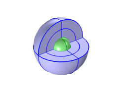
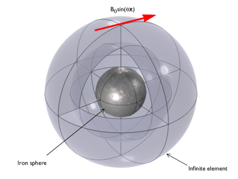
PDF

Iron Sphere in a Magnetic Field — 13.56 MHz
Introduction
This tutorial is part of a series on modeling an iron sphere in a background magnetic field within the Introduction to Electromagnetics tutorial group. This tutorial focuses on the case of a magnetically permeable iron sphere in a spatially uniform magnetic field where the magnetic field sinusoidally varies in time at a frequency of 13.56 MHz. At this frequency, the skin depth of the iron used in the model is ~ 0.65 μm, which is negligible compared to the size of the sphere. In this scenario, we only need to consider surface effects and can model the sphere as an empty shell with an Impedance Boundary Condition.
Model Definition
Figure 1: A magnetically permeable iron sphere in a spatially uniform background magnetic field that sinusoidally varies in time with angular frequency, ω. The sphere at the center is surrounded by air and enclosed in a region of Infinite Elements.
Each model in this tutorial series uses the same basic structure illustrated in Figure 1. It consists of a 0.25 mm diameter iron sphere, with a relative permeability of, μr = 4000, placed in a spatially uniform background magnetic field of strength B0 = 1 mT. In this case, that magnetic field oscillates at a frequency of 13.56 MHz. Due to the negligible skin depth of iron at this frequency, the sphere volume is removed from the Magnetic Fields physics selection and the associated mesh. This saves on computational power. When implemented in this manner, the volume of the sphere is still available to other physics if the user wishes to implement another physics interface (such as Heat Transfer) to model the iron sphere center.
Results and Discussion
The results for this model are shown in Figure 2. The distortion of the background magnetic field is visible along with the distribution of the induced current density across the surface of the iron sphere.
Figure 2: The induced currents on the surface of the iron sphere and the magnetic field in the surrounding space.
Application Library path: ACDC_Module/Introductory_Electromagnetics/iron_sphere_bfield_04_13mhz
Modeling Instructions
This tutorial will demonstrate the physics of an iron sphere in a spatially uniform magnetic field sinusoidally varying at 13.56 MHz. The instructions on the following pages will help you to build, configure, solve, and analyze the model. If anything seems out of order, please retrace your steps. The finalized model — available in the model’s Application Libraries folder — can help you out. You can compare it directly to your current model by means of the Compare option in the Developer toolbar.
Root
The geometry, materials, and selections have been prepared in the Introduction tutorial (chapter 1). They have been saved in the file iron_sphere_bfield_00_introduction.mph. You can start by opening this file and saving it under a new name.
Hint: if you are new to COMSOL Multiphysics, it is worthwhile to check out the Introduction tutorial first.
1
From the File menu, choose Open.
2
3
From the File menu, choose Save As.
4
Magnetic Fields (mf)
As the skin depth is negligible in this model, we are only considering surface effects. This means the volume of the iron sphere can be removed from the physics selection to save on computational cost.
1
In the Model Builder window, under Component 1 (comp1) click Magnetic Fields (mf).
2
In the Settings window for Magnetic Fields, locate the Domain Selection section.
3
4
Click the  Zoom to Selection button in the Graphics toolbar.
Note: In the introduction modeling steps, the nearest upper quarter sphere was hidden to improve visibility in the result plots. This allows the visibility of the mesh layers of the Infinite Element Domain and the Analysis Domain.
5
Click  Remove from Selection.
6
The surface of the sphere is then modeled using an impedance boundary.
Impedance Boundary Condition 1
1
In the Physics toolbar, click  Boundaries and choose Impedance Boundary Condition.
2
In the Settings window for Impedance Boundary Condition, locate the Boundary Selection section.
3
From the Selection list, choose Iron Sphere Surface.
Mesh 1
1
In the Model Builder window, under Component 1 (comp1) click Mesh 1.
2
In the Settings window for Mesh, locate the Sequence Type section.
3
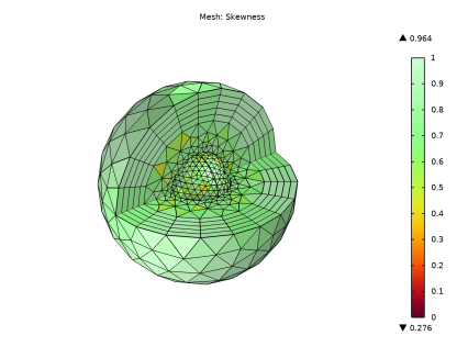
From the list, choose User-controlled mesh.
Size 1
1
In the Model Builder window, right-click Free Tetrahedral 1 and choose Size.
2
In the Settings window for Size, locate the Geometric Entity Selection section.
3
From the Geometric entity level list, choose Boundary.
4
From the Selection list, choose Iron Sphere Surface.
5
Locate the Element Size section. From the Predefined list, choose Extra fine.
6
Click  Build All.
7
In the Mesh toolbar, click  Plot.
Results
Mesh 1
1
Click the  Zoom Extents button in the Graphics toolbar.
The mesh plot shows the details on the surface of the iron sphere but the inner volume is not meshed as it is not included in the physics.
Study 1
Step 1: Frequency Domain
1
In the Model Builder window, expand the Study 1 node, then click Step 1: Frequency Domain.
2
In the Settings window for Frequency Domain, locate the Study Settings section.
3
In the Frequencies text field, type 13.56[MHz].
4
In the Study toolbar, click  Compute.
Results
Magnetic Flux Density (mf)
1
In the Settings window for 3D Plot Group, click to expand the Selection section.
2
From the Geometric entity level list, choose Domain.
3
From the Selection list, choose Analysis domain.
4
Locate the Plot Settings section. Clear the Plot dataset edges checkbox.
5
Locate the Color Legend section. Clear the Show maximum and minimum values checkbox.
6
Select the Show units checkbox.
7
In the Magnetic Flux Density (mf) toolbar, click  Plot.
8
Click the  Zoom Extents button in the Graphics toolbar.
The model has calculated the magnetic flux density in the analysis domain surrounding the iron sphere but there is nothing inside the sphere volume. As the magnetic field is only interacting with the outer shell of the iron sphere using the impedance boundary condition, the current is only induced on the surface.
Surface 1
The final section of this tutorial covers plotting the current density on the surface of the iron sphere and the perturbed background magnetic field. We can also include a material appearance on the surface for completeness.
1
Right-click Magnetic Flux Density (mf) and choose Surface.
2
In the Settings window for Surface, click Replace Expression in the upper-right corner of the Expression section. From the menu, choose Materials > material.boundary - Material settings.
3
Click to expand the Title section. From the Title type list, choose None.
Material Appearance 1
1
Right-click Surface 1 and choose Material Appearance.
2
In the Settings window for Material Appearance, locate the Appearance section.
3
From the Appearance list, choose Custom.
4
From the Material type list, choose Iron (scratched).
Selection 1
1
In the Model Builder window, right-click Surface 1 and choose Selection.
2
In the Settings window for Selection, locate the Selection section.
3
From the Selection list, choose Iron Sphere Surface.
4
In the Magnetic Flux Density (mf) toolbar, click  Plot.
Set the background magnetic field plot to just the horizontal plane.
Multislice 1
1
In the Model Builder window, under Results > Magnetic Flux Density (mf) click Multislice 1.
2
In the Settings window for Multislice, locate the Expression section.
3
From the Unit list, choose mT.
4
Locate the Multiplane Data section. Find the x-planes subsection. Clear the Coordinates text field.
5
Find the y-planes subsection. Clear the Coordinates text field.
Transparency 1
1
Right-click Multislice 1 and choose Transparency.
2
In the Settings window for Transparency, locate the Transparency section.
3
Find the Transparency subsection. In the Transparency text field, type 0.15.
Filter 1
1
Right-click Multislice 1 and choose Filter.
2
In the Settings window for Filter, locate the Element Selection section.
3
In the Logical expression for inclusion text field, type y>0.
Streamline Multislice 1
1
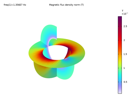
In the Model Builder window, under Results > Magnetic Flux Density (mf) click Streamline Multislice 1.
2
In the Settings window for Streamline Multislice, locate the Multiplane Data section.
3
Find the x-planes subsection. Clear the Coordinates text field.
4
Find the y-planes subsection. Clear the Coordinates text field.
5
Click to expand the Inherit Style section. Clear the Transparency checkbox.
Filter 1
1
In the Model Builder window, expand the Streamline Multislice 1 node, then click Filter 1.
2
In the Settings window for Filter, locate the Element Selection section.
3
In the Logical expression for inclusion text field, type y>0.
4
In the Magnetic Flux Density (mf) toolbar, click  Plot.
Add an arrow surface to visualize the induced current direction.
Arrow Surface 1
1
In the Model Builder window, right-click Magnetic Flux Density (mf) and choose Arrow Surface.
2
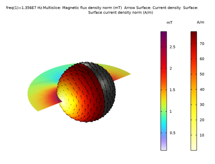
In the Settings window for Arrow Surface, click Replace Expression in the upper-right corner of the Expression section. From the menu, choose Component 1 (comp1) > Magnetic Fields > Currents and charge > mf.Jx,mf.Jy,mf.Jz - Current density.
3
Locate the Arrow Positioning section. From the Placement list, choose Mesh vertices.
4
Locate the Coloring and Style section. From the Color list, choose Black.
Selection 1
1
Right-click Arrow Surface 1 and choose Selection.
2
In the Settings window for Selection, locate the Selection section.
3
From the Selection list, choose Iron Sphere Surface.
4
In the Magnetic Flux Density (mf) toolbar, click  Plot.
5
Click the  Zoom Extents button in the Graphics toolbar.
Surface 2
1
In the Model Builder window, right-click Magnetic Flux Density (mf) and choose Surface.
Show the current density norm on half of the sphere.
2
In the Settings window for Surface, click Replace Expression in the upper-right corner of the Expression section. From the menu, choose Component 1 (comp1) > Magnetic Fields > Currents and charge > mf.normJs - Surface current density norm - A/m.
3
Locate the Coloring and Style section. From the Color table list, choose Thermal.
4
From the Color table transformation list, choose Reverse.
Filter 1
1
Right-click Surface 2 and choose Filter.
2
In the Settings window for Filter, locate the Element Selection section.
3
In the Logical expression for inclusion text field, type x<0.
Selection 1
1
In the Model Builder window, right-click Surface 2 and choose Selection.
2
In the Settings window for Selection, locate the Selection section.
3
From the Selection list, choose Iron Sphere Surface.
4
In the Magnetic Flux Density (mf) toolbar, click  Plot.
This surface plot shows that there is a peak surface current density of ~ 78 A/m around the circumference of the sphere.
This tutorial demonstrated the efficacy of using only the surface of the iron sphere for models using a negligible skin depth. For comparison, the user can investigate and recreate these results using the sphere volume and adding a mesh with a very high detail near the surface. This can be accomplished by constructing a mesh similar to that demonstrated in the 20 kHz oscillating magnetic field tutorial but with an even smaller layer thickness.