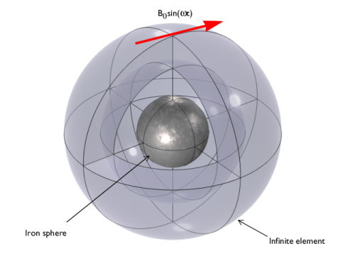
PDF

Iron Sphere in a Magnetic Field — 20 kHz
Introduction
This tutorial is part of a series on modeling an iron sphere in a background magnetic field within the Introduction to Electromagnetics tutorial group. This tutorial focuses on the case of a magnetically permeable iron sphere in a spatially uniform magnetic field where the magnetic field sinusoidally varies in time at a frequency of 20 kHz. At this frequency, the skin depth of the iron used in the model is ~ 17 μm, which means the signal penetrates part-way into the iron sphere.
Model Definition
Figure 1: A magnetically permeable iron sphere in a spatially uniform background magnetic field that sinusoidally varies in time with angular frequency, ω. The sphere at the center is surrounded by air and enclosed in a region of Infinite Elements.
Each model in this tutorial series uses the same basic structure illustrated in Figure 1. It consists of a 0.25 mm diameter iron sphere, with a relative permeability of, μr = 4000, placed in a spatially uniform background magnetic field of strength B0 = 1 mT. In this case, that magnetic field oscillates at a frequency of 20 kHz.
In the current model, the intermediary nature of the skin depth results in a significant amount of detail in the magnetic field and the induced currents near the surface of the sphere. This is modeled by creating a tailored mesh with elements that follow the symmetry of the model and are sufficiently smaller than the scales of interest. The mesh shown in Figure 2 was used to resolve the fine details near the surface of the sphere.
Figure 2: Mesh plot showing the regions of tetrahedral mesh in yellow that make up the majority of the domains of interest and the boundary layers in blue that resolve the detail near the surface of the sphere. The infinite element domain is shown in gray.
Results and Discussion
The magnetic flux density and the induced currents are shown in Figure 3. The magnetic field and current density are strongest near the surface of the sphere.
Figure 3: Cross-section of the iron sphere showing the induced current in the sphere and the magnetic flux.
Application Library path: ACDC_Module/Introductory_Electromagnetics/iron_sphere_bfield_03_20khz
Modeling Instructions
This tutorial will demonstrate the physics of an iron sphere in a spatially uniform magnetic field sinusoidally varying at 20 kHz. The instructions on the following pages will help you to build, configure, solve, and analyze the model. If anything seems out of order, please retrace your steps. The finalized model — available in the model’s Application Libraries folder — can help you out. You can compare it directly to your current model by means of the Compare option in the Developer toolbar.
Root
The geometry, materials, and selections have been prepared in the Introduction tutorial (chapter 1). They have been saved in the file iron_sphere_bfield_00_introduction.mph. You can start by opening this file and saving it under a new name.
Hint: if you are new to COMSOL Multiphysics, it is worthwhile to check out the Introduction tutorial first.
1
From the File menu, choose Open.
2
3
From the File menu, choose Save As.
4
Magnetic Fields (mf)
Free Space 1
To begin, enter the parameters specific for this model. This model uses a stabilization conductivity of 50 S/m.
1
In the Model Builder window, expand the Component 1 (comp1) > Magnetic Fields (mf) node, then click Free Space 1.
2
In the Settings window for Free Space, locate the Stabilization section.
3
From the σstab list, choose User defined. In the associated text field, type 50.
Mesh 1
To begin, we can demonstrate the results produced with the default mesh.
1
In the Model Builder window, under Component 1 (comp1) right-click Mesh 1 and choose Build All.
2
Click the  Zoom to Selection button in the Graphics toolbar.
Note: In the introduction modeling steps, the nearest upper quarter sphere was hidden to improve visibility in the result plots. This allows the visibility of the mesh layers of the Infinite Element Domain and the Analysis Domain.
Study 1
Step 1: Frequency Domain
1
In the Model Builder window, expand the Study 1 node, then click Step 1: Frequency Domain.
2
In the Settings window for Frequency Domain, locate the Study Settings section.
3
In the Frequencies text field, type 20[kHz].
4
In the Study toolbar, click  Compute.
Results
Study 1/Solution 1 (sol1)
In the Model Builder window, expand the Results > Datasets node, then click Study 1/Solution 1 (sol1).
Selection
1
In the Results toolbar, click  Attributes and choose Selection.
2
In the Settings window for Selection, locate the Geometric Entity Selection section.
3
From the Geometric entity level list, choose Domain.
4
From the Selection list, choose Analysis domain.
Magnetic Flux Density (mf)
1
In the Model Builder window, under Results click Magnetic Flux Density (mf).
2
In the Magnetic Flux Density (mf) toolbar, click  Plot.
3
Click the  Zoom Extents button in the Graphics toolbar.
The magnetic flux density within the sphere has not been solved well due to the large magnetic gradients not being resolved by large mesh elements. The next part will go through construction of a more appropriate mesh for the simulation parameters set in this tutorial. To assess the appropriate size of mesh elements for this study, we can refer to the skin depth of the iron sphere under this 20 kHz background magnetic field. This value is uniform across the domain and can be obtained by evaluating the maximum value in the volume.
Volume Maximum 1
1
In the Results toolbar, click  More Derived Values and choose Maximum > Volume Maximum.
2
In the Settings window for Volume Maximum, locate the Selection section.
3
From the Selection list, choose Iron Sphere.
4
Click Replace Expression in the upper-right corner of the Expressions section. From the menu, choose Component 1 (comp1) > Magnetic Fields > Material properties > mf.deltaS - Skin depth - m.
5
Click  Evaluate.
The skin depth of the iron sphere in this case should be 0.0168 mm, so this is the scale of interest for this model. Ideally, the mesh element thickness near the surface of the iron sphere should be smaller than the scale of interest to adequately resolve the magnetic gradients. Also, due to the spherical symmetry of the model, we can use a boundary layer mesh with a thickness smaller than the scale of interest.
Mesh 1
1
In the Model Builder window, under Component 1 (comp1) click Mesh 1.
2
In the Settings window for Mesh, locate the Sequence Type section.
3
From the list, choose User-controlled mesh.
Size 1
1
In the Model Builder window, right-click Free Tetrahedral 1 and choose Size.
2
In the Settings window for Size, locate the Geometric Entity Selection section.
3
From the Selection list, choose Iron Sphere.
4
Locate the Element Size section. From the Predefined list, choose Extra fine.
Boundary Layers 1
1
In the Mesh toolbar, click  Boundary Layers.
2
In the Settings window for Boundary Layers, locate the Geometric Entity Selection section.
3
From the Geometric entity level list, choose Domain.
4
From the Selection list, choose Iron Sphere.
Boundary Layer Properties
1
In the Model Builder window, click Boundary Layer Properties.
2
In the Settings window for Boundary Layer Properties, locate the Boundary Selection section.
3
From the Selection list, choose Iron Sphere Surface.
4
Locate the Layers section. From the Thickness specification list, choose First layer.
5
In the Thickness text field, type 8[um].
6
In the Number of layers text field, type 4.
7
Click  Build All.
8
In the Mesh toolbar, click  Plot.
Results
Mesh 1
1
In the Settings window for Mesh, click to expand the Title section.
2
From the Title type list, choose None.
3
Locate the Level section. From the Element type list, choose Prism.
4
Locate the Coloring and Style section. From the Element color list, choose Cyan.
5
Click to expand the Element Filter section. Select the Enable filter checkbox.
6
In the Expression text field, type z<0.
Selection 1
1
Right-click Mesh 1 and choose Selection.
2
In the Settings window for Selection, locate the Selection section.
3
From the Selection list, choose Analysis domain.
Mesh 2
1
Right-click Mesh 1 and choose Duplicate.
2
In the Settings window for Mesh, locate the Level section.
3
From the Element type list, choose Tetrahedron.
4
Locate the Coloring and Style section. From the Element color list, choose Yellow.
Mesh 3
1
Right-click Mesh 1 and choose Duplicate.
2
In the Settings window for Mesh, locate the Coloring and Style section.
3
From the Element color list, choose Gray.
Selection 1
1
In the Model Builder window, expand the Mesh 3 node, then click Selection 1.
2
In the Settings window for Selection, locate the Selection section.
3
From the Selection list, choose Infinite Element Domain.
Transparency 1
1
In the Model Builder window, right-click Mesh 3 and choose Transparency.
2
In the Mesh Plot 2 toolbar, click  Plot.
3
Click the  Zoom Extents button in the Graphics toolbar.
4
In the Model Builder window, click Transparency 1.
This new mesh has a much finer resolution normal to the surface of the iron sphere, where the steeper magnetic gradients are located. Now, rerun the study and compare the results.
Study 1
In the Study toolbar, click  Compute.
Results
Magnetic Flux Density (mf)
1
In the Magnetic Flux Density (mf) toolbar, click  Plot.
2
Click the  Zoom Extents button in the Graphics toolbar.
The magnetic flux density plotted is now much smoother and has been resolved to a much higher precision. Next, plot the current density induced in the sphere.
Arrow Volume 1
1
Right-click Magnetic Flux Density (mf) and choose Arrow Volume.
2
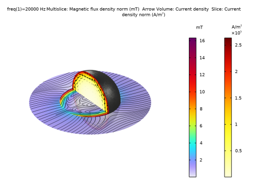
In the Settings window for Arrow Volume, click Replace Expression in the upper-right corner of the Expression section. From the menu, choose Component 1 (comp1) > Magnetic Fields > Currents and charge > mf.Jx,mf.Jy,mf.Jz - Current density.
3
Locate the Arrow Positioning section. Find the x grid points subsection. In the Points text field, type 1.
4
Find the y grid points subsection. In the Points text field, type 15.
5
Find the z grid points subsection. In the Points text field, type 15.
6
Locate the Coloring and Style section. From the Color list, choose Black.
7
Select the Scale factor checkbox. In the associated text field, type 3e-7.
Selection 1
1
Right-click Arrow Volume 1 and choose Selection.
2
In the Settings window for Selection, locate the Selection section.
3
From the Selection list, choose Iron Sphere.
4
In the Magnetic Flux Density (mf) toolbar, click  Plot.
5
Click the  Zoom Extents button in the Graphics toolbar.
Here, it is shown that there is substantial more current induced near the surface of the iron sphere, as expected from the skin depth of iron at this frequency of background magnetic field. We can also evaluate the magnetic dissipation in the iron sphere from the work done on the sphere.
Volume Integration 1
1
In the Results toolbar, click  More Derived Values and choose Integration > Volume Integration.
2
In the Settings window for Volume Integration, locate the Selection section.
3
From the Selection list, choose Iron Sphere.
4
Click Add Expression in the upper-right corner of the Expressions section. From the menu, choose Component 1 (comp1) > Magnetic Fields > Heating and losses > mf.Qrh - Volumetric loss density, electric - W/m³.
5
Click  Evaluate.
In this model, the magnetic dissipation in the sphere is ~3.4 nW.