|
|
|
|
1
|
Use a stabilization conductivity corresponding to a ratio of 1000:1 between the largest and smallest skin depths in the model. In this case, this means using a value of σstab = 5000 S/m. This will add artificial magnetic dissipation in the air domains in the model.
|
|
1
|
|
2
|
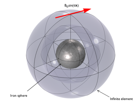
Browse to the model’s Application Libraries folder and double-click the file iron_sphere_bfield_00_introduction.mph.
|
|
3
|
|
4
|
Browse to a suitable folder and type the filename iron_sphere_bfield_02_60hz.mph.
|
|
1
|
In the Model Builder window, expand the Component 1 (comp1) > Magnetic Fields (mf) node, then click Free Space 1.
|
|
2
|
|
3
|
|
1
|
|
2
|
|
3
|
|
4
|
Click
|
|
5
|
|
1
|
|
2
|
|
1
|
In the Model Builder window, expand the Study 1 - Without Gauge Fixing node, then click Step 1: Frequency Domain.
|
|
2
|
|
3
|
|
4
|
|
5
|
Click
|
|
7
|
|
1
|
In the Model Builder window, expand the Results > Datasets node, then click Study 1 - Without Gauge Fixing/Solution 1 (sol1).
|
|
2
|
|
1
|
|
2
|
|
3
|
|
4
|
|
1
|
|
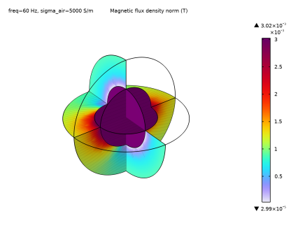
2
|
In the Settings window for 3D Plot Group, type Magnetic Flux Density - Without Gauge Fixing in the Label text field.
|
|
3
|
|
4
|
|
1
|
|
2
|
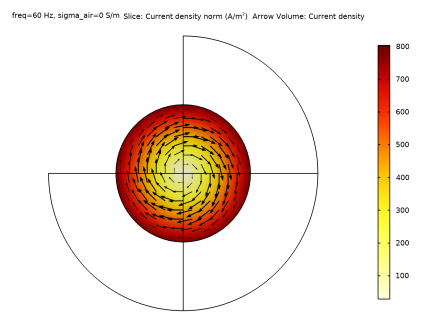
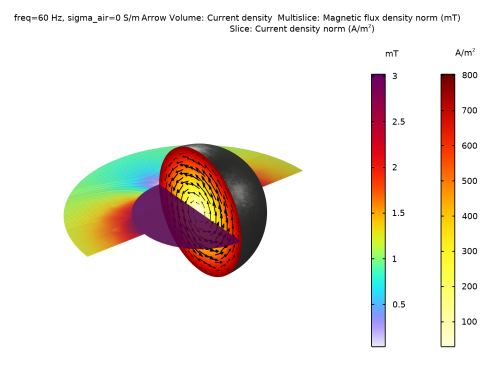
In the Settings window for 3D Plot Group, type Current Density - Without Gauge Fixing in the Label text field.
|
|
3
|
|
4
|
|
1
|
|
2
|
In the Settings window for Slice, click Replace Expression in the upper-right corner of the Expression section. From the menu, choose Component 1 (comp1) > Magnetic Fields > Currents and charge > mf.normJ - Current density norm - A/m².
|
|
3
|
|
4
|
|
5
|
|
6
|
|
1
|
In the Model Builder window, right-click Current Density - Without Gauge Fixing and choose Arrow Volume.
|
|
2
|
In the Settings window for Arrow Volume, click Replace Expression in the upper-right corner of the Expression section. From the menu, choose Component 1 (comp1) > Magnetic Fields > Currents and charge > mf.Jx,mf.Jy,mf.Jz - Current density.
|
|
3
|
Locate the Arrow Positioning section. Find the x grid points subsection. In the Points text field, type 1.
|
|
4
|
|
5
|
|
6
|
|
7
|
|
8
|
|
9
|
|
1
|
|
2
|
|
3
|
|
4
|
Click Replace Expression in the upper-right corner of the Expressions section. From the menu, choose Component 1 (comp1) > Magnetic Fields > Material properties > mf.deltaS - Skin depth - m.
|
|
5
|
Click
|
|
1
|
|
2
|
In the Settings window for Volume Maximum, type Skin Depth - Air (Without Gauge Fixing) in the Label text field.
|
|
3
|
|
4
|
Click Replace Expression in the upper-right corner of the Expressions section. From the menu, choose Component 1 (comp1) > Magnetic Fields > Material properties > mf.deltaS - Skin depth - m.
|
|
5
|
Click
|
|
1
|
|
2
|
In the Settings window for Volume Integration, type Magnetic Dissipation - Iron Sphere in the Label text field.
|
|
3
|
|
4
|
Click Replace Expression in the upper-right corner of the Expressions section. From the menu, choose Component 1 (comp1) > Magnetic Fields > Heating and losses > mf.Qrh - Volumetric loss density, electric - W/m³.
|
|
5
|
Click
|
|
1
|
|
2
|
In the Settings window for Volume Integration, type Dissipation - Air (Without Gauge Fixing) in the Label text field.
|
|
3
|
|
5
|
Click
|
|
7
|
Click Replace Expression in the upper-right corner of the Expressions section. From the menu, choose Component 1 (comp1) > Magnetic Fields > Heating and losses > mf.Qrh - Volumetric loss density, electric - W/m³.
|
|
8
|
Click
|
|
1
|
|
2
|
|
3
|
Select the Modify model configuration for study step checkbox.
|
|
4
|
|
5
|
Right-click and choose Disable.
|
|
1
|
|
2
|
Go to the Add Study window.
|
|
3
|
|
4
|
Click the Add Study button in the window toolbar.
|
|
5
|
|
1
|
|
2
|
|
3
|
|
4
|
Click
|
|
6
|
|
7
|
|
8
|
|
1
|
In the Model Builder window, under Results > Datasets click Study 2 - With Gauge Fixing/Solution 2 (sol2).
|
|
2
|
|
1
|
|
2
|
|
3
|
|
4
|
|
1
|
|
2
|
In the Settings window for 3D Plot Group, type Magnetic Flux Density - With Gauge Fixing in the Label text field.
|
|
3
|
|
1
|
In the Model Builder window, right-click Current Density - Without Gauge Fixing and choose Duplicate.
|
|
2
|
In the Settings window for 3D Plot Group, type Current Density - With Gauge Fixing in the Label text field.
|
|
3
|
|
4
|
|
5
|
|
6
|
|
1
|
|
2
|
In the Settings window for Volume Maximum, type Skin Depth - Air (With Gauge Fixing) in the Label text field.
|
|
3
|
|
4
|
|
5
|
Click Replace Expression in the upper-right corner of the Expressions section. From the menu, choose Component 1 (comp1) > Magnetic Fields > Material properties > mf.deltaS - Skin depth - m.
|
|
6
|
Click
|
|
1
|
|
2
|
In the Settings window for Volume Integration, type Dissipation - Air (With Gauge Fixing) in the Label text field.
|
|
3
|
|
5
|
Click
|
|
7
|
Click Replace Expression in the upper-right corner of the Expressions section. From the menu, choose Component 1 (comp1) > Magnetic Fields > Heating and losses > mf.Qrh - Volumetric loss density, electric - W/m³.
|
|
8
|
|
9
|
Click
|