PDF

Generator in 2D
Introduction
This example shows how the circular motion of a rotor with permanent magnets generates an induced EMF in a stator winding. The generated voltage is calculated as a function of time during the rotation. The model also shows the influence on the voltage from material parameters, rotation velocity, and number of turns in the winding.
The center of the rotor consists of annealed medium carbon steel, which is a material with a high relative permeability. The center is surrounded with several blocks of a permanent magnet made of sintered NdFeB, creating a strong magnetic field. The stator is made of the same permeable material as the center of the rotor, confining the field in closed loops through the winding. The winding is wound around the stator poles. Figure 1 shows the generator with part of the stator sliced in order to show the winding and the rotor.
Figure 1: Drawing of a generator showing how the rotor, stator, and stator winding are constructed. The coils are connected in series in order to give the highest possible voltage.
Modeling in COMSOL Multiphysics
The COMSOL Multiphysics model of the generator is a time-dependent 2D problem on a cross section through the generator. This is a true time-dependent model where the motion of the magnetic sources in the rotor is accounted for in the boundary condition between the stator and rotor geometries. Thus, there is no Lorentz term in the equation, resulting in the PDE
where the magnetic vector potential only has a  z component.
Rotation is modeled using a ready-made physics interface for rotating machinery. The center part of the geometry, containing the rotor and part of the air-gap, rotates relative to the coordinate system of the stator. The rotor and the stator are built as two separate geometry objects, so it is possible to use an assembly (see Finalizing the Geometry in the COMSOL Multiphysics Reference Manual for details). This has several advantages: the coupling between the rotor and the stator is done automatically, the parts are meshed independently, and it allows for a discontinuity in the vector potential at the interface between the two geometry objects (called slits). The rotor problem is solved in a rotating coordinate system where the rotor is fixed (the rotor frame), whereas the stator problem is solved in a coordinate system that is fixed with respect to the stator (the stator frame). An identity pair connecting the rotating rotor frame with the fixed stator frame is created between the rotor and the stator. The identity pair enforces continuity for the vector potential in the global fixed coordinate system (the stator frame).
The stator and center of the rotor are made of annealed medium-carbon steel (soft iron), which is implemented in COMSOL Multiphysics as an interpolation function of the B-H curve of the material; see Figure 2.
Figure 2: The norm of the magnetic flux, |B|, versus the norm of the magnetic field, |H|, for the rotor and stator materials.
The generated voltage is computed automatically with the use of the Coil feature. In this simplified example all coils are connected in series, making out a single stator winding. The series connection of coils is realized in COMSOL Multiphysics by adding coil domains to a Coil group. In this way, the output voltage is the sum of voltages generated by each coil even though they are not geometrically connected in the 2D model.
The resistive and iron losses are computed with the use of a Loss Calculation subfeature and a Time to Frequency Losses study. In this 2D model, the magnets are modeled by using the Coil feature, which allows for the calculation of induced currents and resistive losses. The settings impose a zero net perpendicular current in each of the magnets by activating the Coil group checkbox. For the iron part of the generator, the Bertotti loss model is selected to compute the cycle averaged loss power density. A surface integration is then made to compute the total loss power of the generator. The generated voltage and the losses are compared with the 3D counterpart of this model, that is, Modeling of an Electric Generator in 3D.
Results and Discussion
The generated voltage in the rotor winding is close to a sinusoidal signal. At a rotation speed of 60 rpm the voltage has an amplitude of 700 V in total; see Figure 3.
Figure 3: The generated voltage over one quarter of a revolution. This simulation used a 100-turn winding.
The norm of the magnetic flux density, |B|, and the B field lines are shown below in Figure 4 at the time 0.20 s.
Figure 4: The norm and the field lines of the magnetic flux density after 0.2 s of rotation. Note the darker regions, which indicate the position of the permanent magnets in the rotor.
The cycle averaged losses power density is shown below in Figure 5.
Figure 5: The volumetric loss density of the generator.
Application Library path: ACDC_Module/Devices,_Motors_and_Generators/generator_2d
Modeling Instructions
From the File menu, choose New.
New
In the New window, click  Model Wizard.
Model Wizard
1
In the Model Wizard window, click  2D.
2
In the Select Physics tree, select AC/DC > Electromagnetics and Mechanics > Rotating Machinery, Magnetic (rmm).
3
Click Add.
4
Click  Study.
5
In the Select Study tree, select General Studies > Stationary.
6
Global Definitions
Parameters 1
1
In the Model Builder window, under Global Definitions click Parameters 1.
2
In the Settings window for Parameters, locate the Parameters section.
3
Next, build the generator using rotor and stator parts from the geometry part library. Initialize the parts, and tick the selections that are predefined to make it convenient to assign material properties and magnetization direction.
Part Libraries
1
In the Home toolbar, click  Windows and choose Part Libraries.
2
In the Part Libraries window, select AC/DC Module > Rotating Machinery 2D > Rotors > Internal > surface_mounted_magnet_internal_rotor_2d in the tree.
3
Click  Add to Geometry.
Part Libraries
1
In the Home toolbar, click  Windows and choose Part Libraries.
2
In the Model Builder window, under Component 1 (comp1) click Geometry 1.
3
In the Part Libraries window, select AC/DC Module > Rotating Machinery 2D > Stators > External > slotted_external_stator_2d in the tree.
4
Click  Add to Geometry.
Geometry 1
1
In the Home toolbar, click  Build All.
2
Click the  Zoom Extents button in the Graphics toolbar.
3
In the Model Builder window, under Component 1 (comp1) click Geometry 1.
Internal Rotor – Surface Mounted Magnets 1 (pi1)
1
In the Model Builder window, under Component 1 (comp1) > Geometry 1 click Internal Rotor – Surface Mounted Magnets 1 (pi1).
2
In the Settings window for Part Instance, locate the Input Parameters section.
3
4
Click to expand the Domain Selections section. In the table, enter the following settings:
External Stator – Slotted 1 (pi2)
1
In the Model Builder window, click External Stator – Slotted 1 (pi2).
2
In the Settings window for Part Instance, locate the Input Parameters section.
3
4
Locate the Domain Selections section. In the table, enter the following settings:
Definitions
Iron
1
In the Definitions toolbar, click  Union.
2
In the Settings window for Union, locate the Input Entities section.
3
Under Selections to add, click  Add.
4
In the Add dialog, in the Selections to add list, choose Shaft (Internal Rotor – Surface Mounted Magnets 1), Rotor iron (Internal Rotor – Surface Mounted Magnets 1), and Stator iron (External Stator – Slotted 1).
5
6
In the Settings window for Union, type Iron in the Label text field.
Iron and Magnets
1
In the Definitions toolbar, click  Union.
2
In the Settings window for Union, locate the Input Entities section.
3
Under Selections to add, click  Add.
4
In the Add dialog, in the Selections to add list, choose Iron and Rotor Magnets (Internal Rotor – Surface Mounted Magnets 1).
5
6
In the Settings window for Union, type Iron and Magnets in the Label text field.
Create an assembly from the two geometry objects, connected by a pair boundary.
Geometry 1
Form Union (fin)
1
In the Model Builder window, under Component 1 (comp1) > Geometry 1 click Form Union (fin).
2
In the Settings window for Form Union/Assembly, locate the Form Union/Assembly section.
3
From the Action list, choose Form an assembly.
4
In the Geometry toolbar, click  Build All.
5
Click the  Zoom Extents button in the Graphics toolbar.
6
In the Model Builder window, click Geometry 1.
Add Material
1
In the Materials toolbar, click  Add Material to open the Add Material window.
2
Go to the Add Material window.
3
In the tree, select Built-in > Air.
4
Click the Add to Component button in the window toolbar.
5
In the tree, select AC/DC > Soft Iron (Without Losses).
6
Click the Add to Component button in the window toolbar.
7
In the tree, select AC/DC > Hard Magnetic Materials > Sintered NdFeB Grades (Chinese Standard) > N50 (Sintered NdFeB).
8
Click the Add to Component button in the window toolbar.
9
In the Materials toolbar, click  Add Material to close the Add Material window.
Materials
Soft Iron (Without Losses) (mat2)
1
In the Settings window for Material, locate the Geometric Entity Selection section.
2
From the Selection list, choose Iron.
N50 (Sintered NdFeB) (mat3)
1
In the Model Builder window, click N50 (Sintered NdFeB) (mat3).
2
In the Settings window for Material, locate the Geometric Entity Selection section.
3
From the Selection list, choose Rotor Magnets (Internal Rotor – Surface Mounted Magnets 1).
Rotating Machinery, Magnetic (rmm)
1
In the Model Builder window, under Component 1 (comp1) click Rotating Machinery, Magnetic (rmm).
2
In the Settings window for Rotating Machinery, Magnetic, locate the Thickness section.
3
In the d text field, type L.
Next, use a Rotating Domain feature to specify the rotor’s rotational velocity.
Component 1 (comp1)
Rotating Domain 1
1
In the Physics toolbar, click  Moving Mesh and choose Rotating Domain.
2
In the Settings window for Rotating Domain, locate the Domain Selection section.
3
From the Selection list, choose All domains (Internal Rotor – Surface Mounted Magnets 1).
4
Locate the Rotation section. From the Rotation type list, choose Specified rotational velocity.
5
From the Rotational velocity expression list, choose Constant revolutions per time.
6
In the f text field, type rpm.
To define the remanent flux direction of all magnets, use the Conducting Magnet feature.
Rotating Machinery, Magnetic (rmm)
Conducting Magnet 1
1
In the Physics toolbar, click  Domains and choose Conducting Magnet.
2
In the Settings window for Conducting Magnet, locate the Domain Selection section.
3
From the Selection list, choose Rotor Magnets (Internal Rotor – Surface Mounted Magnets 1).
4
Locate the Magnet section. From the Pattern type list, choose Circular pattern.
5
From the Type of periodicity list, choose Alternating.
North 1
1
In the Model Builder window, click North 1.
2
South 1
1
In the Model Builder window, click South 1.
2
Conducting Magnet 1
In the Model Builder window, click Conducting Magnet 1.
Loss Calculation 1
In the Physics toolbar, click  Attributes and choose Loss Calculation.
Iron
1
In the Physics toolbar, click  Domains and choose Ampère’s Law.
2
In the Settings window for Ampère’s Law, locate the Constitutive Relation B-H section.
3
From the Magnetization model list, choose B-H curve.
4
Locate the Domain Selection section. From the Selection list, choose Iron.
5
In the Label text field, type Iron.
Add the Loss Calculation subfeature to compute iron losses.
Loss Calculation 1
1
In the Physics toolbar, click  Attributes and choose Loss Calculation.
Set loss model to Bertotti.
2
In the Settings window for Loss Calculation, locate the Loss Model section.
3
From the Loss model list, choose Bertotti.
Domain Coil 1
1
In the Physics toolbar, click  Domains and choose Domain Coil.
2
In the Settings window for Domain Coil, locate the Domain Selection section.
3
From the Selection list, choose Stator slots (External Stator – Slotted 1).
4
Locate the Coil section. From the Conductor model list, choose Homogenized multiturn.
5
In the Icoil text field, type 0[A].
6
Locate the Homogenized Conductor section. In the N text field, type N.
7
From the Coil wire cross-section area list, choose From diameter.
8
In the d text field, type d_wire.
9
Locate the Coil section. Select the Coil group checkbox.
Reversed Current Direction 1
1
In the Physics toolbar, click  Attributes and choose Reversed Current Direction.
2
Study 1
Step 2: Time Dependent
1
In the Study toolbar, click  Time Dependent.
2
In the Settings window for Time Dependent, locate the Study Settings section.
3
In the Output times text field, type range(0,0.005,0.25).
Before solving refine the mesh on boundaries associated with the Continuity condition for more accurate results.
Definitions
Identity Boundary Pair 1 (ap1)
1
In the Model Builder window, under Component 1 (comp1) > Definitions click Identity Boundary Pair 1 (ap1).
2
In the Settings window for Pair, locate the Source Boundaries section.
3
Click  Create Selection.
4
In the Create Selection dialog, type source in the Selection name text field.
5
6
In the Settings window for Pair, locate the Destination Boundaries section.
7
Click  Create Selection.
8
In the Create Selection dialog, type destination in the Selection name text field.
9
Airgap Boundaries
1
In the Definitions toolbar, click  Union.
2
In the Settings window for Union, type Airgap Boundaries in the Label text field.
3
Locate the Geometric Entity Level section. From the Level list, choose Boundary.
4
Locate the Input Entities section. Under Selections to add, click  Add.
5
In the Add dialog, in the Selections to add list, choose source and destination.
6
Mesh 1
Free Triangular 1
In the Mesh toolbar, click  Free Triangular.
Size
1
In the Model Builder window, click Size.
2
In the Settings window for Size, locate the Element Size section.
3
From the Predefined list, choose Coarser.
4
Click the Custom button.
5
Locate the Element Size Parameters section. In the Maximum element size text field, type 0.015.
Size 1
1
In the Model Builder window, right-click Free Triangular 1 and choose Size.
2
In the Settings window for Size, locate the Geometric Entity Selection section.
3
From the Geometric entity level list, choose Boundary.
4
From the Selection list, choose Airgap Boundaries.
5
Locate the Element Size section. From the Predefined list, choose Extremely fine.
6
Click  Build All.
Study 1
In the Study toolbar, click  Compute.
Postprocessing the Results
Now, plot the solution in the spatial frame (the stator’s fixed frame) at the time t = 0.2 s.
1
In the Settings window for 2D Plot Group, locate the Data section.
2
From the Time (s) list, choose 0.2.
3
In the Magnetic Flux Density (rmm) toolbar, click  Plot.
Figure 4 shows the rotor position at t = 0.2 s, as well as the magnetic flux density norm and magnetic flux density lines. Next, plot the induced EMF in a quarter of the cycle.
Induced Coil Voltage
1
In the Results toolbar, click  1D Plot Group.
2
In the Settings window for 1D Plot Group, type Induced Coil Voltage in the Label text field.
3
Click to expand the Title section. From the Title type list, choose Manual.
4
In the Title text area, type Induced voltage.
5
Locate the Plot Settings section.
6
Select the x-axis label checkbox. In the associated text field, type Time (s).
7
Select the y-axis label checkbox. In the associated text field, type Voltage (V).
Global 1
1
Right-click Induced Coil Voltage and choose Global.
2
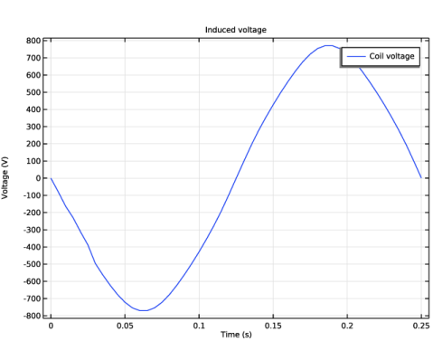
In the Settings window for Global, click Replace Expression in the upper-right corner of the y-Axis Data section. From the menu, choose Component 1 (comp1) > Rotating Machinery, Magnetic (Magnetic Fields) > Coil parameters > rmm.VCoil_1 - Coil voltage - V.
3
In the Induced Coil Voltage toolbar, click  Plot.
The resulting plot is Figure 3.
Next, add the Time to Frequency Losses study to compute the iron loss.
Add Study
1
In the Home toolbar, click  Add Study to open the Add Study window.
2
Go to the Add Study window.
3
Find the Studies subsection. In the Select Study tree, select Preset Studies for Selected Physics Interfaces > Time-to-Frequency Losses.
4
Click the Add Study button in the window toolbar.
5
In the Home toolbar, click  Add Study to close the Add Study window.
Study 2
Step 1: Time-to-Frequency Losses
1
In the Settings window for Time-to-Frequency Losses, locate the Study Settings section.
2
From the Input study list, choose Study 1, Time Dependent.
3
In the Electrical period text field, type 0.25.
4
In the Study toolbar, click  Compute.
Results
Cycle Averaged Losses (rmm)
The resulting plot is Figure 5.
Finally, compute the total iron loss power.
Surface Integration 1
1
In the Results toolbar, click  More Derived Values and choose Integration > Surface Integration.
2
In the Settings window for Surface Integration, locate the Data section.
3
From the Dataset list, choose Study 2/Solution 3 (sol3).
4
Locate the Selection section. From the Selection list, choose Iron and Magnets.
5
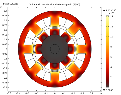
Click Replace Expression in the upper-right corner of the Expressions section. From the menu, choose Component 1 (comp1) > Rotating Machinery, Magnetic (Magnetic Fields, No Currents) > Heating and losses > rmm.Qh - Volumetric loss density, electromagnetic - W/m³.
6
Locate the Expressions section. In the table, enter the following settings:
7
Click  Evaluate.
The computed total loss power is about 455 W.