|
|
|
|
1
|
|
2
|
|
3
|
Click Add.
|
|
4
|
In the Select Physics tree, select Mathematics > ODE and DAE Interfaces > Global ODEs and DAEs (ge).
|
|
5
|
Click Add.
|
|
6
|
Click
|
|
7
|
|
8
|
Click
|
|
1
|
|
2
|
|
1
|
|
2
|
|
3
|
|
1
|
|
2
|
|
3
|
|
4
|
|
5
|
|
6
|
Click
|
|
1
|
|
2
|
|
3
|
|
4
|
|
5
|
Click
|
|
1
|
|
2
|
|
3
|
|
4
|
|
5
|
|
6
|
|
7
|
Click
|
|
8
|
|
1
|
|
2
|
|
3
|
|
4
|
|
5
|
|
6
|
|
7
|
Click
|
|
1
|
|
2
|
|
3
|
|
4
|
|
5
|
|
6
|
|
7
|
Clear the Layers on bottom checkbox.
|
|
9
|
Click
|
|
1
|
|
2
|
|
1
|
|
3
|
|
1
|
|
3
|
|
1
|
|
2
|
|
3
|
|
4
|
|
5
|
|
1
|
|
2
|
|
1
|
|
2
|
|
3
|
|
4
|
|
5
|
|
1
|
|
2
|
|
1
|
|
3
|
|
4
|
|
1
|
In the Model Builder window, under Component 1 (comp1) > Global ODEs and DAEs (ge) click Global Equations 1 (ODE1).
|
|
2
|
|
4
|
|
5
|
|
6
|
|
7
|
Click OK.
|
|
8
|
|
9
|
Click
|
|
10
|
|
11
|
|
12
|
Click OK.
|
|
1
|
|
1
|
|
2
|
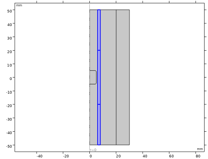
In the Settings window for Ampère’s Law in Solids, type Ampère's Law - Magnet in the Label text field.
|
|
3
|
|
4
|
Locate the Constitutive Relation B-H section. From the Magnetization model list, choose Remanent flux density.
|
|
5
|
Specify the e vector as
|
|
1
|
|
2
|
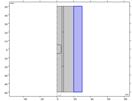
In the Settings window for Ampère’s Law in Solids, type Ampère's Law - Copper Tube in the Label text field.
|
|
3
|
|
1
|
|
2
|
|
3
|
|
4
|
|
1
|
|
1
|
|
2
|
Go to the Add Material window.
|
|
3
|
|
4
|
Right-click and choose Add to Component 1 (comp1).
|
|
5
|
In the tree, select AC/DC > Hard Magnetic Materials > Sintered NdFeB Grades (Chinese Standard) > N50 (Sintered NdFeB).
|
|
6
|
Right-click and choose Add to Component 1 (comp1).
|
|
7
|
|
1
|
|
2
|
|
1
|
|
2
|
|
3
|
|
1
|
|
2
|
|
3
|
Clear the Generate default plots checkbox.
|
|
1
|
|
2
|
|
3
|
In the Solve for column of the table, under Component 1 (comp1), clear the checkbox for Global ODEs and DAEs (ge).
|
|
1
|
|
2
|
|
3
|
|
4
|
|
5
|
|
6
|
|
1
|
|
2
|
|
1
|
|
2
|
|
3
|
|
4
|
|
1
|
|
2
|
|
1
|
|
2
|
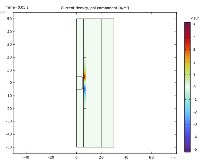
In the Settings window for Surface, click Replace Expression in the upper-right corner of the Expression section. From the menu, choose Component 1 (comp1) > Magnetic Fields > Currents and charge > Current density - A/m² > mf.Jphi - Current density, phi-component.
|
|
3
|
|
4
|
|
1
|
|
2
|
|
1
|
|
2
|
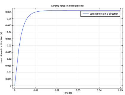
In the Settings window for Global, click Replace Expression in the upper-right corner of the y-Axis Data section. From the menu, choose Component 1 (comp1) > Definitions > Variables > Fz - Lorentz force in z direction - N.
|
|
3
|
|
4
|
Click
|
|
1
|
|
2
|
|
1
|
|
2
|
|
4
|
|
1
|
|
2
|
|
1
|
|
2
|
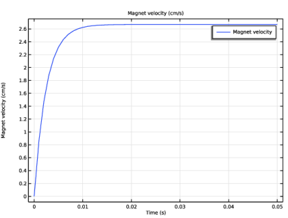
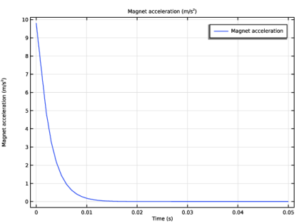
In the Settings window for Global, click Replace Expression in the upper-right corner of the y-Axis Data section. From the menu, choose Component 1 (comp1) > Definitions > Variables > a - Magnet acceleration - m/s².
|
|
3
|