|
|
|


|
1
|
|
2
|
|
3
|
Click Add.
|
|
4
|
In the Select Physics tree, select Mathematics > ODE and DAE Interfaces > Boundary ODEs and DAEs (bode).
|
|
5
|
Click Add.
|
|
6
|
Click
|
|
7
|
In the Select Study tree, select Preset Studies for Selected Physics Interfaces > Electric Currents > Small-Signal Analysis, Frequency Domain.
|
|
8
|
Click
|
|
1
|
|
2
|
|
3
|
Locate the Parameters section. In the table, enter the following settings:
|
|
1
|
|
2
|
|
3
|
Locate the Parameters section. In the table, enter the following settings:
|
|
1
|
|
2
|
|
3
|
Locate the Parameters section. In the table, enter the following settings:
|
|
1
|
|
2
|
|
3
|
|
4
|
|
5
|
|
6
|
|
7
|
|
8
|
Click to expand the Layers section. In the table, enter the following settings:
|
|
1
|
|
2
|
|
3
|
|
4
|
|
5
|
|
1
|
|
2
|
|
3
|
|
1
|
|
2
|
|
3
|
On the object fin, select Domains 2 and 4 only.
|
|
1
|
|
2
|
On the object fin, select Domain 3 only.
|
|
3
|
|
4
|
Click
|
|
1
|
|
2
|
On the object fin, select Domain 1 only.
|
|
3
|
|
1
|
|
2
|
On the object fin, select Domains 1 and 3 only.
|
|
3
|
In the Settings window for Explicit Selection, type Intra/Extracellular Domains in the Label text field.
|
|
1
|
|
2
|
|
3
|
|
4
|
|
5
|
On the object fin, select Boundaries 12 and 13 only.
|
|
1
|
|
2
|
|
3
|
|
4
|
|
5
|
On the object fin, select Boundaries 11 and 14 only.
|
|
1
|
|
2
|
|
3
|
|
4
|
On the object fin, select Boundary 8 only.
|
|
5
|
|
1
|
|
2
|
|
3
|
|
4
|
|
5
|
On the object fin, select Boundary 2 only.
|
|
1
|
|
2
|
|
3
|
In the Settings window for General Extrusion, type Mapping from Intracellular to Extracellular in the Label text field.
|
|
4
|
|
5
|
|
6
|
|
7
|
Locate the Destination Map section. In the r-expression text field, type r/sqrt(r^2+z^2)*(r_cell-t_m).
|
|
8
|
|
9
|
|
1
|
|
2
|
In the Settings window for General Extrusion, type Mapping from Extracellular to Intracellular in the Label text field.
|
|
3
|
|
4
|
|
5
|
|
6
|
|
7
|
|
8
|
|
1
|
|
2
|
|
3
|
Locate the Geometric Entity Selection section. From the Geometric entity level list, choose Boundary.
|
|
4
|
|
5
|
Locate the Variables section. In the table, enter the following settings:
|
|
1
|
|
2
|
|
3
|
|
4
|
|
5
|
|
6
|
Locate the Variables section. In the table, enter the following settings:
|
|
1
|
|
2
|
|
3
|
|
4
|
|
5
|
|
6
|
|
1
|
In the Model Builder window, under Component 1 (comp1) > Electric Currents (ec) click Current Conservation in Solids 1.
|
|
2
|
In the Settings window for Current Conservation in Solids, type Current Conservation - Membrane in the Label text field.
|
|
3
|
|
1
|
|
2
|
|
3
|
|
4
|
|
5
|
|
1
|
|
2
|
In the Settings window for Current Conservation in Solids, type Current Conservation - Intra/Extracellular in the Label text field.
|
|
3
|
|
4
|
|
1
|
|
2
|
|
3
|
|
4
|
|
5
|
|
1
|
|
2
|
|
3
|
|
1
|
|
2
|
In the Settings window for Boundary Terminal, type Terminal for Small-Signal Analysis, Frequency Domain in the Label text field.
|
|
3
|
|
4
|
|
1
|
|
2
|
|
3
|
|
1
|
|
2
|
|
3
|
|
4
|
|
5
|
|
6
|
|
1
|
|
2
|
In the Settings window for Boundary Terminal, type Terminal for Time Dependent in the Label text field.
|
|
3
|
|
4
|
|
5
|
|
1
|
|
2
|
|
3
|
|
4
|
|
5
|
In the Dependent variable quantity table, enter the following settings:
|
|
6
|
In the Source term quantity table, enter the following settings:
|
|
7
|
|
8
|
In the Dependent variables (1/m²) table, enter the following settings:
|
|
1
|
In the Model Builder window, under Component 1 (comp1) > Boundary ODEs and DAEs (bode) click Distributed ODE 1.
|
|
2
|
|
3
|
|
1
|
|
2
|
|
3
|
|
1
|
In the Model Builder window, under Component 1 (comp1) right-click Materials and choose Blank Material.
|
|
2
|
|
3
|
|
4
|
|
5
|
Locate the Material Contents section. In the table, enter the following settings:
|
|
1
|
|
2
|
|
3
|
|
4
|
|
5
|
Locate the Material Contents section. In the table, enter the following settings:
|
|
1
|
|
2
|
|
3
|
|
4
|
|
5
|
Locate the Material Contents section. In the table, enter the following settings:
|
|
1
|
|
2
|
|
1
|
|
2
|
|
1
|
|
2
|
|
1
|
|
1
|
|
2
|
|
3
|
|
4
|
Select the Equidistant checkbox.
|
|
1
|
|
2
|
|
3
|
|
1
|
|
2
|
|
3
|
Clear the Generate default plots checkbox.
|
|
1
|
|
2
|
|
3
|
Select the Modify model configuration for study step checkbox.
|
|
4
|
In the tree, select Component 1 (comp1) > Electric Currents (ec) > Terminal for Stationary Before Time Dependent and Component 1 (comp1) > Electric Currents (ec) > Terminal for Time Dependent.
|
|
5
|
Click
|
|
1
|
|
2
|
|
3
|
|
4
|
Locate the Physics and Variables Selection section. Select the Modify model configuration for study step checkbox.
|
|
5
|
In the tree, select Component 1 (comp1) > Electric Currents (ec) > Terminal for Stationary Before Time Dependent and Component 1 (comp1) > Electric Currents (ec) > Terminal for Time Dependent.
|
|
6
|
Click
|
|
7
|
|
1
|
|
2
|
Go to the Add Study window.
|
|
3
|
|
4
|
Click the Add Study button in the window toolbar.
|
|
1
|
|
2
|
Select the Modify model configuration for study step checkbox.
|
|
3
|
|
4
|
Click
|
|
1
|
|
2
|
|
3
|
|
1
|
|
2
|
|
3
|
In the Model Builder window, under Study 2 > Solver Configurations > Solution 3 (sol3) click Time-Dependent Solver 1.
|
|
4
|
|
5
|
|
6
|
|
7
|
|
8
|
Clear the Generate default plots checkbox.
|
|
9
|
|
1
|
|
2
|
|
3
|
|
4
|
|
5
|
|
1
|
|
2
|
|
3
|
|
4
|
|
5
|
|
1
|
|
2
|
|
3
|
|
4
|
|
1
|
|
2
|
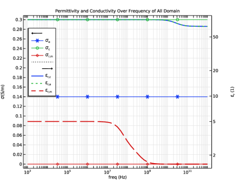
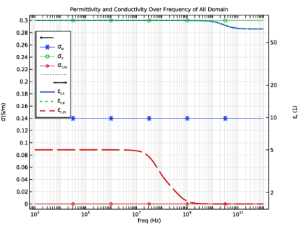
In the Settings window for 1D Plot Group, type Permittivity and Conductivity Spectra in the Label text field.
|
|
3
|
|
4
|
|
5
|
Click to collapse the Title section. Locate the Plot Settings section. Select the x-axis label checkbox.
|
|
6
|
Select the y-axis label checkbox.
|
|
7
|
Select the Two y-axes checkbox.
|
|
8
|
|
9
|
|
10
|
Select the Secondary y-axis label checkbox. In the associated text field, type \varepsilon<SUB>r</SUB> (1).
|
|
1
|
|
3
|
|
4
|
|
5
|
|
6
|
|
7
|
|
8
|
|
9
|
|
1
|
In the Model Builder window, right-click Permittivity and Conductivity Spectra and choose Point Graph.
|
|
2
|
|
3
|
|
4
|
|
5
|
|
6
|
Locate the Coloring and Style section. Find the Line style subsection. From the Line list, choose Cycle.
|
|
7
|
|
8
|
|
9
|
|
11
|
|
12
|
|
1
|
|
2
|
|
3
|
Click to select the
|
|
5
|
|
6
|
Locate the Coloring and Style section. Find the Line markers subsection. From the Marker list, choose Cycle.
|
|
7
|
|
8
|
|
9
|
|
10
|
|
11
|
Select the Show legends checkbox.
|
|
1
|
|
2
|
|
3
|
|
4
|
|
5
|
Locate the Coloring and Style section. Find the Line markers subsection. From the Marker list, choose Cycle.
|
|
6
|
|
7
|
|
8
|
|
9
|
|
11
|
|
12
|
|
1
|
|
2
|
|
3
|
|
4
|
|
5
|
|
6
|
|
7
|
|
1
|
|
2
|
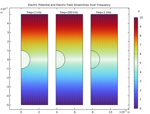
In the Settings window for 2D Plot Group, type Electric Potential (Frequency Domain) in the Label text field.
|
|
3
|
|
4
|
|
5
|
Clear the Parameter indicator text field.
|
|
6
|
|
7
|
|
1
|
|
2
|
|
3
|
|
4
|
|
5
|
|
6
|
|
1
|
In the Model Builder window, right-click Electric Potential (Frequency Domain) and choose Streamline.
|
|
2
|
|
3
|
|
4
|
|
5
|
|
6
|
|
7
|
|
8
|
|
9
|
|
10
|
|
11
|
Clear the Color checkbox.
|
|
1
|
|
2
|
|
3
|
Clear the Color legend checkbox.
|
|
4
|
|
1
|
|
2
|
|
3
|
|
1
|
In the Model Builder window, under Results > Electric Potential (Frequency Domain) right-click Surface 1 and choose Duplicate.
|
|
2
|
|
3
|
|
4
|
|
5
|
|
1
|
In the Model Builder window, under Results > Electric Potential (Frequency Domain) right-click Streamline 1 and choose Duplicate.
|
|
2
|
|
3
|
|
4
|
|
1
|
In the Model Builder window, under Results > Electric Potential (Frequency Domain) right-click Surface 2 and choose Duplicate.
|
|
2
|
|
3
|
|
4
|
|
1
|
In the Model Builder window, under Results > Electric Potential (Frequency Domain) right-click Streamline 2 and choose Duplicate.
|
|
2
|
|
3
|
|
4
|
|
1
|
In the Model Builder window, expand the Electric Potential (Frequency Domain) node, then click Annotation 1.
|
|
2
|
|
3
|
|
4
|
|
5
|
|
6
|
|
7
|
|
8
|
|
9
|
|
1
|
|
2
|
|
3
|
|
4
|
|
1
|
|
2
|
|
3
|
|
4
|
|
5
|
|
6
|
|
1
|
|
2
|
|
3
|
|
4
|
|
5
|
|
6
|
|
7
|
|
8
|
Select the x-axis label checkbox.
|
|
9
|
Select the y-axis label checkbox.
|
|
10
|
Select the Secondary y-axis label checkbox.
|
|
11
|
|
12
|
|
13
|
|
14
|
|
15
|
Select the y-axis log scale checkbox.
|
|
16
|
|
1
|
|
2
|
|
3
|
Click to select the
|
|
5
|
|
6
|
|
8
|
Select the Show legends checkbox.
|
|
1
|
|
3
|
|
4
|
|
5
|
|
6
|
|
8
|
Select the Show legends checkbox.
|
|
9
|
|
10
|
|
11
|
|
1
|
|
2
|
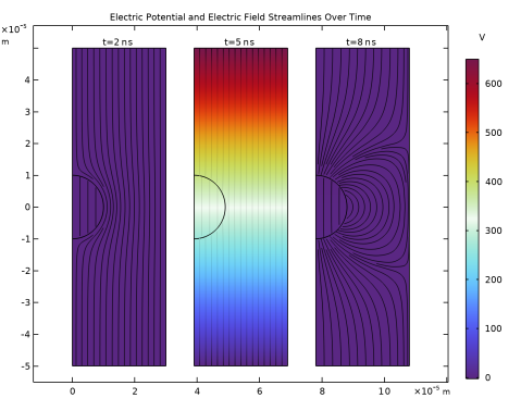
In the Settings window for 2D Plot Group, type Electric Potential (Time Dependent) in the Label text field.
|
|
3
|
|
4
|
|
5
|
Clear the Parameter indicator text field.
|
|
6
|
|
7
|
|
8
|
|
1
|
|
2
|
|
3
|
Select the Manual indexing checkbox.
|
|
4
|
|
5
|
|
6
|
|
7
|
|
1
|
|
2
|
|
3
|
|
4
|
|
5
|
|
6
|
|
7
|
|
8
|
|
9
|
Click to collapse the Inherit Style section. Click to expand the Inherit Style section. From the Plot list, choose Surface 1.
|
|
10
|
Clear the Color checkbox.
|
|
11
|
|
1
|
|
2
|
|
3
|
Clear the Color legend checkbox.
|
|
4
|
|
1
|
|
2
|
|
3
|
|
4
|
|
1
|
In the Model Builder window, under Results > Electric Potential (Time Dependent) right-click Surface 1 and choose Duplicate.
|
|
2
|
|
3
|
|
4
|
|
5
|
|
1
|
In the Model Builder window, under Results > Electric Potential (Time Dependent) right-click Streamline 1 and choose Duplicate.
|
|
2
|
|
3
|
|
4
|
|
1
|
In the Model Builder window, under Results > Electric Potential (Frequency Domain), Ctrl-click to select Annotation 1, Annotation 2, and Annotation 3.
|
|
2
|
Right-click and choose Copy.
|
|
1
|
|
2
|
|
1
|
|
2
|
|
3
|
|
1
|
|
2
|
|
3
|
|
4
|
|
5
|
|
1
|
|
2
|
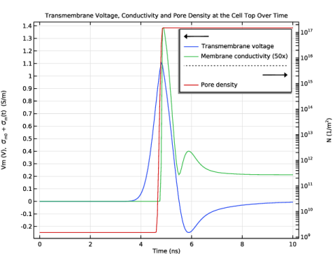
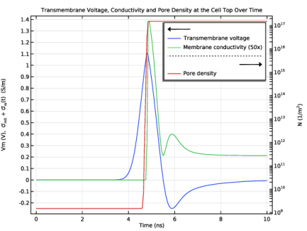
In the Settings window for 1D Plot Group, type Voltage, Conductivity and Pore Density in the Label text field.
|
|
3
|
|
4
|
|
5
|
In the Title text area, type Transmembrane Voltage, Conductivity and Pore Density at the Cell Top Over Time.
|
|
6
|
|
7
|
Select the y-axis label checkbox.
|
|
8
|
Select the Two y-axes checkbox.
|
|
9
|
Select the Secondary y-axis label checkbox.
|
|
10
|
|
11
|
|
12
|
|
13
|
|
1
|
|
3
|
|
4
|
|
5
|
|
6
|
|
7
|
|
1
|
In the Model Builder window, right-click Voltage, Conductivity and Pore Density and choose Point Graph.
|
|
3
|
|
4
|
|
5
|
|
6
|
|
7
|
|
1
|
|
3
|
|
4
|
|
5
|
|
6
|
|
7
|
|
9
|
Select the Show legends checkbox.
|
|
10
|
|
11
|
|
1
|
|
2
|
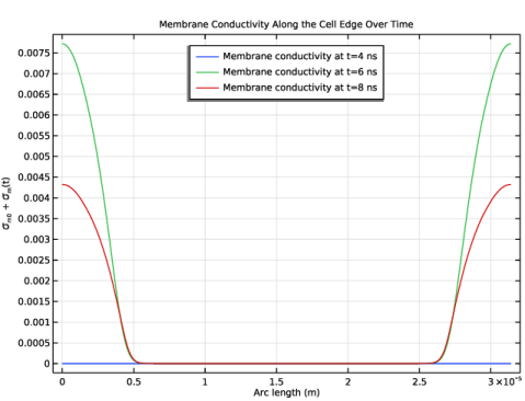
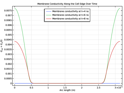
In the Settings window for 1D Plot Group, type Membrane Conductivity Profile in the Label text field.
|
|
3
|
|
4
|
|
5
|
|
6
|
|
7
|
|
8
|
|
9
|
Select the y-axis label checkbox.
|
|
10
|
|
11
|
|
12
|
|
1
|
|
3
|
|
4
|
|
5
|
|
6
|
|
7
|
|
8
|
|
9
|
|
1
|
|
2
|
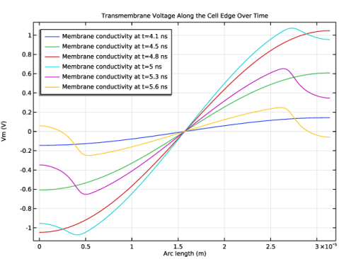
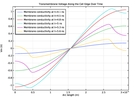
In the Settings window for 1D Plot Group, type Transmembrane Voltage Profile in the Label text field.
|
|
3
|
|
4
|
|
5
|
|
6
|
|
7
|
|
8
|
|
9
|
Select the y-axis label checkbox.
|
|
10
|
|
11
|
|
12
|
|
1
|
|
3
|
|
4
|
|
5
|
|
6
|
|
7
|
|
8
|
|
9
|
|
1
|
|
2
|
|
3
|
|
4
|
|
5
|
|
6
|
|
7
|
|
1
|
|
2
|
|
3
|
|
4
|
|
5
|
|
6
|
|
7
|
|
8
|
|
9
|