PDF

Axisymmetric Approximation of 3D Inductor
Introduction
When the frequency is high enough, capacitative effects can become important also for devices that are inductive and/or resistive at lower frequencies. Modeling this effect in an inductor requires accounting for electric field components both parallel and perpendicular to the wire. This easily leads to the conclusion that a 3D model is always necessary even if the coil is a low slant helix. This is not always the case, as shown in this tutorial.
Starting from the 3D inductor model described in the Introduction to AC/DC Module manual, a 2D axisymmetric model able to describe a self resonating inductor is created. In order to build an equivalent 2D axisymmetric model, an effective axisymmetric core is drawn and the RLC Coil Group feature is used.
The method shown here is particularly suitable for studying systems with thousands of turns, such as sensors or transformers, with limited computational power.
Model Definition
The 3D solution of the power inductor of Figure 1 is presented in the manual Introduction to AC/DC Module. We are considering the same system.
Figure 1: The 3D geometry representation of the power inductor under study.
In that device, the coil can be treated, to a reasonable level of approximation, as axisymmetric. Therefore, any of its cross-sections are suitable for performing a 2D axisymmetric analysis from a geometric point of view.
On the other hand, the core geometry shape indicates that a 3D analysis is required. However, in order to have a description that is correct from a magnetic point of view, the core does not have to be rotationally symmetric as long as
Such a construction, that is, replacing the 3D core with a 2D axisymmetric representation that preserves the crucial area that influences the magnetic circuit, is shown in Figure 2.
Figure 2: The 2D axisymmetric geometry equivalent to the power inductor under study.
The parameters are defined in Table 1. The original external column area (as given by the Outer column section area variable in Table 1) is the area represented in Figure 3. It is set exactly to in the 2D axisymmetric geometry. Some parameters are directly measured from the original 3D geometry such as the Outer column internal radius and the Upper magnetic circuit closure.
The coil geometry representation in 2D axial symmetry is directly taken from the midplane cross section in the xz-plane in 3D. Figure 4 shows the final 2D axisymmetric geometry.
The main challenge of the 2D axisymmetric coil model is to account for the way that the electric currents will flow. The RLC Coil Group feature available in the Magnetic and Electric Fields interface automatically takes into account that the currents are balanced among
1
2
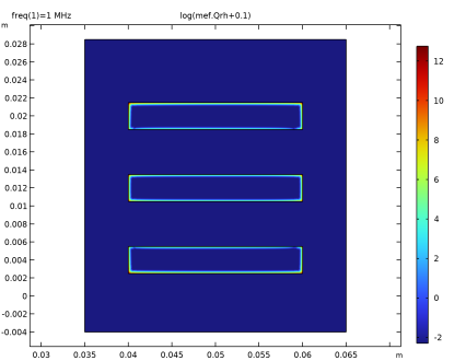
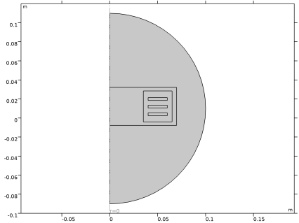
displacement currents that flow in the rz-plane from one turn to the other
In the low-frequency limit, currents are all of the first type. In the high-frequency limit, the currents are all of the second type. At some intermediate frequency there is a resonant frequency where inductive and capacitive effects perfectly balance and the coil self-resonates. At this frequency the inductor is purely resistive and the total loss peaks as a function of frequency.
In this model the core is not grounded and there is no other external electric ground. Compared to a real system where the inductor often is mounted on or near a ground plane, this may cause a shift in the resonance frequency. This is easily added, for example by applying one or more electric boundary conditions to the core boundaries.
Figure 3: The 3D cross sectional area of the outer columns used to compute the 2D axisymmetric outer columns width.
Figure 4: The 2D axisymmetric geometry including some surrounding air.
Results and Discussion
The field and loss plots can be compared to the 3D model discussed in the Introduction to AC/DC Module manual.
Figure 5: Magnetic flux density in the revolved 2D geometry.
Figure 6: The eddy current losses are shown (log scale with zero offset).
The in-plane electric field magnitude strongly depends on the frequency, as is clearly shown from comparing Figure 7 and Figure 8.
Figure 7: Electric field between turns far from the resonance frequency.
Figure 8: Electric field between turns at the resonance frequency.
The most striking sign of the resonance is shown in Figure 9, where the real and imaginary parts of the coil impedance are shown. The resistance (blue curve) is shown in tens of kΩ together with the reactance divided by the angular frequency (green curve). The green curve starts at low frequencies from the static inductance, grows, and then becomes negative. When the green curve becomes negative, it means that the coil behaves like a capacitor. The real part of the impedance accounts for losses, and peaks at the frequency where the capacitative and the inductive contributions to the overall system impedance balance out. The position and value of the peak featured by the 2D axisymmetric model also match the ones of the original 3D model in the Introduction to AC/DC Module manual fairly well.
Figure 9: The inductor impedance as a function of frequency. Compare this plot to the corresponding plot of the 3D Inductor in the Introduction to AC/DC Module manual.
Application Library path: ACDC_Module/Devices,_Inductive/axisymmetric_approximation_of_inductor_3d
Modeling Instructions
From the File menu, choose New.
New
In the New window, click  Model Wizard.
Model Wizard
1
In the Model Wizard window, click  2D Axisymmetric.
2
In the Select Physics tree, select AC/DC > Electromagnetic Fields > Vector Formulations > Magnetic and Electric Fields (mef).
3
Click Add.
4
In the Added physics interfaces tree, select Magnetic and Electric Fields (mef).
5
Click  Study.
6
In the Select Study tree, select General Studies > Frequency Domain.
7
First import the 3D geometry and take some measurements to generate the axisymmetric equivalent.
Part 1
In the Model Builder window, right-click Global Definitions and choose Geometry Parts > 3D Part.
Import 1 (imp1)
1
In the Geometry toolbar, click  Import.
2
In the Settings window for Import, locate the Source section.
3
Click  Browse.
4
5
Click  Import.
Work Plane 1 (wp1)
1
In the Geometry toolbar, click  Work Plane.
2
In the Settings window for Work Plane, locate the Plane Definition section.
3
From the Plane list, choose xz-plane.
4
Click  Go to Plane Geometry.
Work Plane 1 (wp1) > Cross Section 1 (cro1)
1
In the Work Plane toolbar, click  Cross Section.
2
In the Settings window for Cross Section, click  Build Selected.
Work Plane 1 (wp1)
1
In the Model Builder window, under Global Definitions > Geometry Parts > Part 1 click Work Plane 1 (wp1).
2
In the Settings window for Work Plane, click  Build Selected.
Delete Entities 1 (del1)
1
In the Model Builder window, right-click Part 1 and choose Delete Entities.
2
In the Settings window for Delete Entities, locate the Entities or Objects to Delete section.
3
From the Geometric entity level list, choose Domain.
4
On the object imp1, select Domains 2–5 only.
5
Click the  Zoom Extents button in the Graphics toolbar.
6
Click  Build Selected.
Work Plane 2 (wp2)
1
In the Geometry toolbar, click  Work Plane.
2
In the Settings window for Work Plane, locate the Plane Definition section.
3
In the z-coordinate text field, type 5[mm].
4
Click  Go to Plane Geometry.
Work Plane 2 (wp2) > Cross Section 1 (cro1)
1
In the Work Plane toolbar, click  Cross Section.
2
In the Settings window for Cross Section, click  Build Selected.
Work Plane 2 (wp2)
1
In the Model Builder window, under Global Definitions > Geometry Parts > Part 1 click Work Plane 2 (wp2).
2
In the Settings window for Work Plane, click  Build Selected.
Work Plane 3 (wp3)
1
In the Geometry toolbar, click  Work Plane.
2
In the Settings window for Work Plane, locate the Plane Definition section.
3
From the Plane type list, choose Face parallel.
4
On the object del1, select Boundary 46 only.
5
Click  Go to Plane Geometry.
Work Plane 3 (wp3) > Cross Section 1 (cro1)
1
In the Work Plane toolbar, click  Cross Section.
2
In the Settings window for Cross Section, click  Build Selected.
Global Definitions
Add parameters for drawing the axisymmetric equivalent core.
Parameters 1
1
In the Model Builder window, under Global Definitions click Parameters 1.
2
In the Settings window for Parameters, locate the Parameters section.
3
Geometry 1
Import 1 (imp1)
1
In the Model Builder window, under Component 1 (comp1) right-click Geometry 1 and choose Import.
2
In the Settings window for Import, locate the Source section.
3
From the Source list, choose Geometry sequence.
4
From the Geometry list, choose Work Plane 3 (wp3), Part 1.
5
Click Import.
Distance Measurement 1 (dm1)
1
In the Geometry toolbar, click  Measurements and choose Distance Measurement.
Next, make some measurements to use when creating the axisymmetric geometry.
2
On the object imp1(2), select Point 7 only.
3
In the Settings window for Distance Measurement, locate the Geometric Entity Selection section.
4
Click to select the  Activate Selection toggle button for Second entity.
5
On the object imp1(2), select Point 3 only.
Distance Measurement 2 (dm2)
1
In the Geometry toolbar, click  Measurements and choose Distance Measurement.
2
On the object imp1(2), select Point 7 only.
3
In the Settings window for Distance Measurement, locate the Geometric Entity Selection section.
4
Click to select the  Activate Selection toggle button for Second entity.
5
On the object imp1(2), select Point 8 only.
Now that the measures have been stored, delete the part.
Delete Entities 1 (del1)
1
In the Model Builder window, right-click Geometry 1 and choose Delete Entities.
2
In the Settings window for Delete Entities, locate the Entities or Objects to Delete section.
3
Click to select the  Activate Selection toggle button for Selection.
4
From the Geometric entity level list, choose Object.
5
Click the  Select All button in the Graphics toolbar.
6
Click  Build Selected.
Next, repeat the same procedure for another measurement.
Import 2 (imp2)
1
In the Geometry toolbar, click  Import.
2
In the Settings window for Import, locate the Source section.
3
From the Source list, choose Geometry sequence.
4
From the Geometry list, choose Work Plane 2 (wp2), Part 1.
5
Click Import.
Distance Measurement 3 (dm3)
1
In the Geometry toolbar, click  Measurements and choose Distance Measurement.
2
On the object imp2(2), select Point 13 only.
3
In the Settings window for Distance Measurement, locate the Geometric Entity Selection section.
4
Click to select the  Activate Selection toggle button for Second entity.
5
On the object imp2(2), select Point 6 only.
Delete Entities 2 (del2)
1
Right-click Geometry 1 and choose Delete Entities.
2
In the Settings window for Delete Entities, locate the Entities or Objects to Delete section.
3
Click to select the  Activate Selection toggle button for Selection.
4
From the Geometric entity level list, choose Object.
5
Click the  Select All button in the Graphics toolbar.
6
Click  Build Selected.
Now import the last part and use the stored measures to finalize the 2D axisymmetric geometry.
Import 3 (imp3)
1
In the Geometry toolbar, click  Import.
2
In the Settings window for Import, locate the Source section.
3
From the Source list, choose Geometry sequence.
4
From the Geometry list, choose Work Plane 1 (wp1), Part 1.
5
Click Import.
Rectangle 1 (r1)
1
In the Geometry toolbar, click  Rectangle.
2
In the Settings window for Rectangle, locate the Size and Shape section.
3
In the Width text field, type sqrt(external_area/pi+(geom1.dm3/2)^2).
4
In the Height text field, type 0.0325+2*(geom1.dm1*geom1.dm2)/pi/(geom1.dm3/2).
5
Locate the Position section. In the z text field, type -0.004-(geom1.dm1*geom1.dm2)/pi/(geom1.dm3/2).
Intersection 1 (int1)
1
In the Geometry toolbar, click  Booleans and Partitions and choose Intersection.
2
Click in the Graphics window and then press Ctrl+A to select both objects.
3
In the Settings window for Intersection, click  Build Selected.
Circle 1 (c1)
1
In the Geometry toolbar, click  Circle.
2
In the Settings window for Circle, locate the Size and Shape section.
3
In the Radius text field, type 0.1.
4
Locate the Position section. In the z text field, type 0.01.
5
Locate the Size and Shape section. In the Sector angle text field, type 180.
6
Locate the Rotation Angle section. In the Rotation text field, type -90.
Form Union (fin)
1
In the Geometry toolbar, click  Build All.
2
Click the  Zoom Extents button in the Graphics toolbar.
3
In the Model Builder window, click Form Union (fin).
Magnetic and Electric Fields (mef)
Ampère’s Law and Current Conservation in Solids 1
1
In the Physics toolbar, click  Domains and choose Ampère’s Law and Current Conservation in Solids.
2
3
In the Settings window for Ampère’s Law and Current Conservation in Solids, locate the Constitutive Relation B-H section.
4
From the Magnetization model list, choose Magnetic losses.
Magnetic Insulation 1
In the Model Builder window, click Magnetic Insulation 1.
Electric Insulation 1
1
In the Physics toolbar, click  Attributes and choose Electric Insulation.
2
Click the  Select All button in the Graphics toolbar.
First add an Ampère’s Law feature, which is necessary for adding the RLC Coil Group feature.
Ampère’s Law 1
1
In the Physics toolbar, click  Domains and choose Ampère’s Law.
2
Add the RLC Coil Group feature, which takes care of coupling the transverse currents inside the conductors to the capacitative current flowing perpendicularly to the windings.
RLC Coil Group 1
1
In the Physics toolbar, click  Domains and choose RLC Coil Group.
2
As the coils are connected from the bottom to the top and domain ordering is not the same, a manual ordering is necessary.
3
In the Settings window for RLC Coil Group, locate the Geometry section.
4
From the Domain ordering list, choose Manual.
5
Locate the Domain Selection section. In the list box, select 5.
6
Locate the Geometry section. In the Domain list text field, type 5, 4, 6.
In order to improve variable scaling, set a ground voltage slightly different from zero.
7
Locate the RLC Coil Group section. In the V0 text field, type 1[mV].
Materials
Add material data for the copper windings and the lossy iron core.
Material 1 (mat1)
1
In the Model Builder window, under Component 1 (comp1) right-click Materials and choose Blank Material.
2
3
In the Settings window for Material, locate the Material Contents section.
4
Material 2 (mat2)
1
Right-click Materials and choose Blank Material.
2
3
In the Settings window for Material, locate the Material Contents section.
4
Mesh 1
Free Triangular 1
1
In the Mesh toolbar, click  Free Triangular.
2
In the Settings window for Free Triangular, locate the Domain Selection section.
3
From the Geometric entity level list, choose Domain.
4
Size 1
1
Right-click Free Triangular 1 and choose Size.
2
3
In the Settings window for Size, locate the Element Size section.
4
Click the Custom button.
5
Locate the Element Size Parameters section.
6
Select the Maximum element size checkbox. In the associated text field, type 2e-3.
Size 2
1
In the Model Builder window, right-click Free Triangular 1 and choose Size.
2
In the Settings window for Size, locate the Geometric Entity Selection section.
3
Click  Clear Selection.
4
5
Locate the Element Size section. Click the Custom button.
6
Locate the Element Size Parameters section.
7
Select the Maximum element size checkbox. In the associated text field, type 5e-4.
Free Triangular 2
1
In the Mesh toolbar, click  Free Triangular.
2
In the Settings window for Free Triangular, click  Build Selected.
Boundary Layers 1
1
In the Mesh toolbar, click  Boundary Layers.
2
In the Settings window for Boundary Layers, locate the Domain Selection section.
3
From the Geometric entity level list, choose Domain.
4
A boundary layer mesh is added in order to resolve the skin depth.
Boundary Layer Properties
1
In the Model Builder window, click Boundary Layer Properties.
2
In the Settings window for Boundary Layer Properties, locate the Boundary Selection section.
3
From the Selection list, choose All boundaries.
4
Locate the Layers section. From the Thickness specification list, choose First layer.
5
In the Number of layers text field, type 12.
6
In the Stretching factor text field, type 1.3.
7
In the Thickness text field, type 10[um].
8
Click  Build Selected.
Study 1
Step 1: Frequency Domain
1
In the Model Builder window, under Study 1 click Step 1: Frequency Domain.
2
In the Settings window for Frequency Domain, locate the Study Settings section.
3
From the Frequency unit list, choose MHz.
4
In the Frequencies text field, type range(1,0.25,10).
5
In the Study toolbar, click  Compute.
Results
Magnetic Flux Density (mef)
Click the  Zoom Extents button in the Graphics toolbar.
Study 1/Solution 1 (sol1)
In the Model Builder window, expand the Results > Datasets node, then click Study 1/Solution 1 (sol1).
Selection
1
In the Results toolbar, click  Attributes and choose Selection.
2
In the Settings window for Selection, locate the Geometric Entity Selection section.
3
From the Geometric entity level list, choose Domain.
4
Magnetic Flux Density, Revolved Geometry (mef)
In the Model Builder window, under Results click Magnetic Flux Density, Revolved Geometry (mef).
Study 1/Solution 1 (2) (sol1)
In the Results toolbar, click  More Datasets and choose Solution.
Selection
1
In the Results toolbar, click  Attributes and choose Selection.
2
In the Settings window for Selection, locate the Geometric Entity Selection section.
3
From the Geometric entity level list, choose Domain.
4
Resistive Losses
1
In the Results toolbar, click  2D Plot Group.
2
In the Settings window for 2D Plot Group, type Resistive Losses in the Label text field.
3
Locate the Data section. From the Dataset list, choose Study 1/Solution 1 (2) (sol1).
4
From the Parameter value (freq (MHz)) list, choose 1.
Surface 1
1
Right-click Resistive Losses and choose Surface.
2
In the Settings window for Surface, locate the Expression section.
3
In the Expression text field, type log(mef.Qrh+0.1).
4
In the Resistive Losses toolbar, click  Plot.
5
Click the  Zoom Extents button in the Graphics toolbar.
Electric Field
1
In the Results toolbar, click  2D Plot Group.
2
In the Settings window for 2D Plot Group, type Electric Field in the Label text field.
3
Locate the Data section. From the Dataset list, choose Study 1/Solution 1 (2) (sol1).
Arrow Surface 1
1
Right-click Electric Field and choose Arrow Surface.
2
In the Settings window for Arrow Surface, locate the Coloring and Style section.
3
From the Arrow length list, choose Normalized.
4
From the Arrow base list, choose Center.
5
6
In the Scale factor text field, type 3.0E-10.
7
Click the  Zoom Extents button in the Graphics toolbar.
8
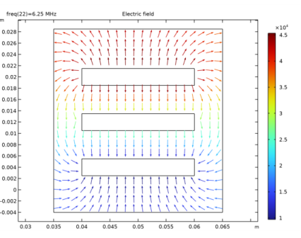
Locate the Arrow Positioning section. Find the r grid points subsection. In the Points text field, type 20.
9
Find the z grid points subsection. In the Points text field, type 20.
10
Click Replace Expression in the upper-right corner of the Expression section. From the menu, choose Component 1 (comp1) > Magnetic and Electric Fields > Electric > mef.Er,mef.Ez - Electric field.
Color Expression 1
1
Right-click Arrow Surface 1 and choose Color Expression.
2
In the Electric Field toolbar, click  Plot.
3
Click the  Zoom Extents button in the Graphics toolbar.
4
In the Model Builder window, click Color Expression 1.
Electric Field
1
In the Model Builder window, under Results click Electric Field.
2
In the Settings window for 2D Plot Group, locate the Data section.
3
From the Parameter value (freq (MHz)) list, choose 6.25.
4
In the Electric Field toolbar, click  Plot.
Impedance
1
In the Results toolbar, click  1D Plot Group.
2
In the Settings window for 1D Plot Group, type Impedance in the Label text field.
3
Click to expand the Title section. From the Title type list, choose None.
4
Locate the Legend section. From the Position list, choose Upper left.
5
Locate the Plot Settings section. Select the Two y-axes checkbox.
Generate a plot with the real and the imaginary part of the impedance, which can be read at low frequency as impedance and resistance. The resonant peak is clearly visible and compares well with the original 3D geometry.
Global 1
Right-click Impedance and choose Global.
Global 2
In the Model Builder window, right-click Impedance and choose Global.
Global 1
1
In the Settings window for Global, locate the y-Axis Data section.
2
Global 2
1
In the Model Builder window, click Global 2.
2
In the Settings window for Global, locate the y-Axis section.
3
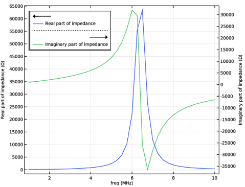
Select the Plot on secondary y-axis checkbox.
4
Locate the y-Axis Data section. In the table, enter the following settings:
5
In the Impedance toolbar, click  Plot.
6
Click the  Zoom Extents button in the Graphics toolbar.