
|
1
|
|
2
|
In the Select Physics tree, under Fluid Flow > Nonisothermal Flow > Rotating Machinery, Nonisothermal Flow click Laminar Flow
|
|
3
|
Click the Add button.
|
|
4
|
|
5
|
|
6
|
|
1
|
|
2
|
Browse to the module’s applications folder and double-click the file nonisothermal_mixer.mph.
|
|
3
|
Go to the Home toolbar and select Build All
|
|
4
|
|
1
|
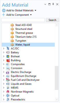
Go to the Add Material window.
|
|
2
|
|
3
|
|
1
|
Go to the Add Material window.
|
|
2
|
|
3
|
|
4
|
|
5
|
|
6
|
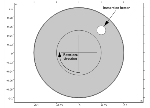
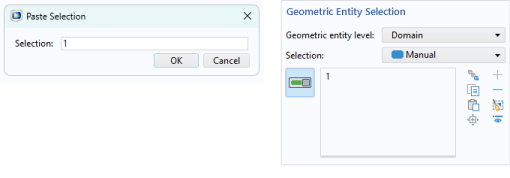
In the settings window for Steel AISI 4340, locate the Geometric Entity Selection section. Select Domain 1, the circular outer rim of the mixer, only.
|
|
1
|
|
1
|
|
2
|
|
3
|
|
4
|
|
5
|
|
1
|
|
2
|
|
3
|
|
4
|
|
1
|
|
1
|
|
1
|
|
1
|
|
3
|
|
4
|
|
1
|
|
3
|
|
4
|
|
5
|
|
6
|
|
1
|
|
2
|
|
3
|
|
1
|
|
2
|
|
3
|
|
4
|
|
1
|
|
2
|
|
3
|
|
5
|
|
6
|
|
8
|
|
1
|
|
2
|
|
3
|
|
4
|
|
1
|
|
2
|
|
3
|
|
4
|
|
5
|
|
6
|
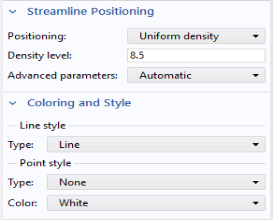
Locate the Coloring and Style section. Find the Point style subsection. From the Color list, choose White.
|
|
7
|
|
8
|
|
1
|
|
2
|
|
3
|
|
4
|
|
5
|
|
6
|
|
7
|
|
8
|
Locate the Coloring and Style section. Find the Point style subsection. From the Color list, choose Gray.
|
|
9
|
|
1
|
|
2
|
|
3
|
|
4
|
|
5
|
|
6
|
|
7
|
|
8
|
|
9
|
Click to expand the Table and Window Settings section. From the Plot window list, choose New window.
|
|
1
|
|
2
|
Go to the Add Study window.
|
|
3
|
|
4
|
|
5
|
|
1
|
|
2
|
|
3
|
|
4
|
Click to expand the Values of Dependent Variables section. Find the Initial values of variables solved for subsection. From the Settings list, choose User controlled.
|
|
5
|
|
6
|
|
1
|
|
2
|
In the Model Builder window, expand the Solution 2 (sol2) node, then click Time-Dependent Solver 1
|
|
3
|
|
4
|
|
5
|
|
6
|
|
1
|
|
2
|
|
3
|
|
1
|
|
2
|
|
3
|
|
1
|
|
2
|
|
3
|
|
4
|
|
5
|
Locate the Coloring and Style section. Find the Point style subsection. From the Color list, choose Gray.
|
|
1
|
|
2
|
|
3
|
|
4
|
|
5
|
|
6
|
|
7
|