About the Mixer Module
The development of new products and processing lines continuously places high demands on mixer design. The Mixer Module provides engineers and scientists with the necessary simulation tools for predicting and understanding the interactions between fluid flow and chemical processes in mixers and stirred vessels.
Figure 1-1: Water free surface in a partially baffled mixer with a three-bladed impeller.
The Mixer Module complements the CFD Module with additional functionality for the Rotating Machinery, Fluid Flow branch. The added functionality includes extended capability for modeling turbulence in the Rotating Machinery interfaces.
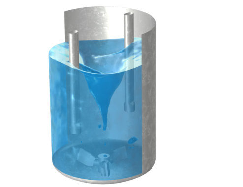
In order to facilitate fast and efficient setup of mixer geometries, the Mixer Module Part Library includes predefined geometry components typical of mixer equipment. The part library includes impeller parts for axial impellers, radial impellers, and impellers designed for highly viscous fluids. In addition to impellers, three types of different tank geometries and a cylindrical impeller shaft geometry are available in the part library. All mixer parts are modularized through a number of input parameters corresponding to important geometrical properties of each part. These parameters can be adjusted in order to fit the mixer system under investigation.
A high rotation rate or a strong acceleration of the rotation rate may induce a substantial deformation of the free surface in an open vessel. This topology change in turn influences the flow pattern inside the vessel. The Mixer Module includes free-surface features to capture the displacement of the liquid-air interface induced by the bulk motion in the domain, by the walls, and by the rotating shaft.
The physics interfaces define a fluid-flow problem using physical quantities such as pressure, flow rate, temperature, and species composition, as well as physical properties, such as viscosity, thermal diffusivity, and density. The different physics interfaces cover a wide range of laminar and turbulent mixer flows. The conservation laws formulated by the physics interfaces are expressed in terms of partial differential equations along with corresponding initial and boundary conditions. The equations are solved by the module using stabilized finite element formulations for fluid flow in combination with damped Newton methods and, for time-dependent problems, in combination with various time-dependent solver algorithms. The Mixer Module’s general capabilities include frozen-rotor, with or without mixing planes applied at boundaries between nonrotating and rotating domains, and time-dependent flows in two- and three-dimensional spaces. For a so-called frozen-rotor flow, the topology relative to the rotating reference frame is fixed (“frozen”). When the flow field is, or can be approximated to be, of this type the computational time (CPU time) can be substantially reduced using the Frozen Rotor (see the CFD Module User’s Guide) study type. The mixing-plane condition models the overall influence of the rotating and nonrotating configurations on the flow field by averaging flow quantities in the direction of rotation.
The workflow in the Mixer Module is quite straightforward. Set up a simulation using one of the Rotating Machinery interfaces, described by the following steps: define the geometry, select the fluid to be modeled, select the type of flow, define the rotating parts, define boundary and initial conditions, define the finite element mesh, select a solver, compute the solution, and visualize the results. All these steps are performed from the COMSOL Desktop. The mesh and solver steps are usually carried out automatically using default settings, which are tuned specifically for each Fluid Flow interface.
The models available in the Mixer Module application library describe the physics interfaces and their features through examples for different types of mixer flows. Here you find examples of industrial equipment and devices, tutorial models for practice, and benchmark models for verification and validation of the Fluid Flow interfaces. Go to The Application Libraries Window to access these resources.
To help you get started, this introduction contains a list of the physics interfaces and an example, Tutorial Model — Nonisothermal Mixer, to introduce you to the workflow.
Aspects of Mixer Simulations
In the initial stages of development for a product, or a new process line, the focus usually lies on qualitative results such as determining whether or not the flow is well mixed, whether a heated reactor is free from hotspots, or whether the flow field contains recirculation zones, which can be inaccessible to reactants. Qualitative results such as these are usually the first step toward creating or improving a design. During the later stages of development, the focus shifts toward scale-up and optimization. For mixing of pseudoplastic slurries, for example, the yield stress has to be overcome everywhere. Bioreactors, on the other hand, should not contain regions of excessive shear. Obtaining accurate estimates for the yield stress, shear, or other process parameters such as reaction rates, thermal equilibration times, torque, and energy consumption, provides developers with the edge needed to assume a competitive position within their field.
The choice of which physics to include in your simulations can be based on experimental results, experience, or a dimensional analysis. Excluding relevant physics undoubtedly leads to wrong results, while including “everything” leads to excessive computational time. The Rotating Machinery interfaces help you set up problems of varying complexity. If the mixed quantity is passive, you can use one of the Rotating Machinery, Fluid Flow interfaces to solve for the fluid flow, and then add a Transport of Diluted Species interface to determine other properties, for example, the mixing efficiency. Both reactions and thermal variations affect constitutive quantities, such as the density and viscosity of the fluid. When these effects become appreciable, you can switch to the Rotating Machinery, Reacting Flow interfaces or the Rotating Machinery, Nonisothermal Flow interfaces. When working with Mach numbers larger than 0.3, you can switch to the Rotating Machinery, High-Mach Number Flow interfaces. When the mixed quantity consists of particles droplets or bubbles, possibly with a different density and response time compared to the surrounding fluid, you can switch to the Rotating Machinery, Multiphase Flow interfaces. In flows with many particles or droplets immersed in a liquid, use the Rotating Machinery, Mixture Model or Rotating Machinery, Phase Transport Mixture Model interfaces. If you are interested in the exact motion of individual bubbles, including how the fluid interface deforms due to, for instance, surface tension, use either the Rotating Machinery, Two-Phase Flow, Level Set or the Rotating Machinery, Two-Phase Flow, Phase Field interfaces. Taking it one step further, COMSOL Multiphysics lets you add other physics interfaces to preexisting ones to tailor simulations to your application.
The physics interfaces in the Mixer Module are able to perform all steps in mixer analyses, from the initial idea and qualitative simulations to the final optimization of the product or process.