The interfaces between phases are tracked with specific boundary conditions for the mesh displacement and the fluid flow. Two options are available — Free Surface and Fluid–Fluid Interface. The Free Surface boundary condition is appropriate when the viscosity of the external fluid is negligible compared to that of the internal fluid. In this case the pressure of the external fluid is the only parameter required to model the fluid and the flow is not solved for in the external fluid. For a fluid-fluid interface the flow is solved for both phases.

The boundary conditions applied at an interface between two immiscible fluids, fluid 1 and fluid 2 (see Figure 4-2), are given by (Ref. 1):

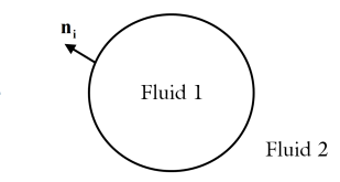
where u1 and u2 are the velocities of the fluids 1 and 2 respectively, umesh is the velocity of the mesh at the interface between the two fluids, ni is the normal of the interface (outward from the domain of fluid 1), τ1 and τ2 are the total stress tensors in domains 1 and 2 respectively, fst is the force per unit area due to the surface tension and Mf is the mass flux across the interface (SI unit: kg/(m2s)).

The tangential components of Equation 4-19 enforce a no-slip condition between the fluids at the boundary. In the absence of mass transfer across the boundary, Equation 4-19 and Equation 4-21 ensure that the fluid velocity normal to the boundary is equal to the velocity of the interface. When mass transfer occurs these equations result from conservation of mass and are easily derived in the frame where the boundary is stationary.

The components of the total stress tensor, τuv, represent the uth component of the force per unit area perpendicular to the v direction. n·τ = nvτuv (using the summation convention) is therefore interpreted as the force per unit area acting on the boundary - in general this is not normal to the boundary. Equation 4-20 therefore expresses the force balance on the interface between the two fluids.

where ∇s is the surface gradient operator (∇s = (I − ni niT)∇, where I is the identity matrix) and σ is the surface tension at the interface.

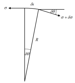
In the two dimensional case it is straightforward to see the physical origin of Equation 4-22. Consider an element of the surface of unit depth into the page as shown in Figure 4-3. The normal force per unit area Fn on the element in the limit δs → 0 is:

Because Rδθ → δs in the limit,

The quantity ∇s·ni in the first term on the right-hand side of Equation 4-22 is related to the mean curvature, κ, of the surface by the equation κ=−∇s·ni. In two dimensions the mean curvature κ = −1/R so ∇s·ni = 1/R. The first term in Equation 4-22 is therefore the normal force per unit area acting on the boundary due to the surface tension.

The tangential force per unit area, Ft, acting on the interface in Figure 4-3 can be obtained from the force balance along the direction of δs in the limit δs → 0:

This is equivalent to the second term on the right of Equation 4-22.

To obtain additional insight into the boundary condition, it is helpful to rewrite Equation 4-20 as

assuming Newtonian fluids with viscosities μ1 and μ2 for fluids 1 and 2, respectively, and that p1 and p2 are the pressures in the respective fluids adjacent to the boundary. This equation expresses the equality of two vector quantities. It is instructive to consider the components perpendicular and tangential to the boundary. In the direction of the boundary normal

whereas in the tangential direction, ti,

For the case of a static interface, Equation 4-23 expresses the pressure difference across the interface that results from its curvature. For a moving interface, the surface tension balances the difference in the total normal stress on either side of the interface.

Equation 4-24 involves only velocity gradients and the gradient of the surface tension. The implication of this is that surface tension gradients always drive motion; this is known as the Marangoni effect.

It is often the case that the viscosity of fluid 1 is significantly greater than that of fluid 2 (for example for a liquid-vapor interface). In this case, the viscosity terms in the total stress from fluid 2 can be neglected and Equation 4-20 becomes:

The outer fluid (fluid 2) now enters the equation system only through the pressure term and the system can be represented by a domain consisting solely of the fluid 1 domain with an expression (or constant value) for the external pressure, pext, in the fluid 2 domain. Since the velocity in fluid 2 does not affect fluid 1, fluid 2 does not need to be explicitly modeled and Equation 4-19 can be dropped.