Results
Add another surface dataset that points to the new solution.
Datasets
1
2
Velocity (Coupled Flow)
Recreate the velocity, pressure, and concentration plots for the fully coupled problem.
1
2
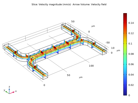
In the Settings window for 3D Plot Group, type Velocity (Coupled Flow) in the Label text field.
3
4
There are significant differences in the flow pattern, although these are hard to see when comparing this plot with the similar one generated previously. The flow through a slice of the channel will be investigated in more detail later to better highlight these differences.
Pressure (Coupled Flow)
1
2
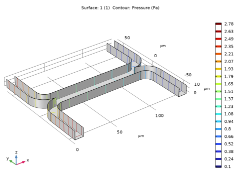
In the Settings window for 3D Plot Group, type Pressure (Coupled Flow) in the Label text field.
3
4
The pressure distribution in the channel has changed significantly as a result of the increased viscosity of the fluid that contains the added species. Thus the two inlets must be maintained at different pressures. This may be possible for a single stage, but it would significantly complicate the design of a multiple stage device.
Concentration (Coupled Flow)
1
2
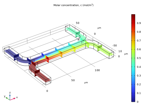
In the Settings window for 3D Plot Group, type Concentration (Coupled Flow) in the Label text field.
3
4
The concentration distribution is affected only slightly by the coupling between the flow and the concentration.
Next add a cut plane dataset in the center of the channel, for both the uncoupled and fully coupled solutions. These will be used to visualize the change in the flow profile induced by the coupling.
Datasets
1
2
3
4
Velocity Comparison
Add a 2D contour plot of the velocity magnitude.
1
2
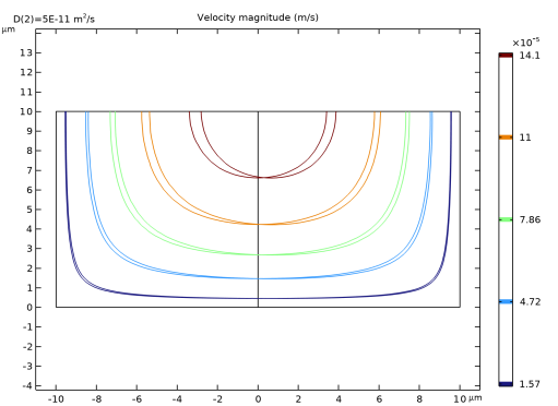
In the Settings window for 2D Plot Group, type Velocity Comparison in the Label text field.
3
-
-
From the Parameter value (D (m2/s)) list, choose 5e-11.
4
5
Create a duplicate contour plot, using the same colors and scales, but showing the coupled data.
6
7
8
9
10
11
12
Now it is possible to compare the velocity distributions more carefully. It is clear that the coupling has introduced an asymmetry into the flow pattern as a result of the higher viscosity in the fluid containing the dissolved species.
Finally compare the output concentration between the two solutions.
Global Evaluation 1
1
2
3
When the diffusion coefficient is 5×10-11 m2/s the mean concentration at the outlet is 0.448 mol/m2.
Global Evaluation 2
1
2
3
Only a small difference occurs in the output concentration as a result of the coupling between the problems. However, the coupling would make adding multiple stages of the device together much more difficult, as different pressures are required at the two inlets to obtain the same flow velocity in the two streams.