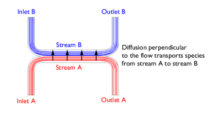
This example treats an H-shaped microfluidic device for separation through diffusion. The device puts two different laminar streams in contact for a controlled period of time. The contact surface is well defined, and by controlling the flow rate it is possible to control the amount of species transported from one stream to the other through diffusion. The device concept is illustrated in Figure 4. The design aims to maintain a laminar flow field when the two streams, A and B, are united and thus prevent uncontrolled convective mixing. The transport of species between streams A and B should take place only by diffusion in order that species with low diffusion coefficients stay in their respective streams. In this way, light species with high diffusivity can be separated from heavy species with low diffusivity. Let us look at a mixture of light and heavy species entering through inlet A. If the separator is properly designed, the heavy species should exit almost exclusively though outlet A. The lighter species should exit through both outlet A and B in equal rates. In this way, outlet B contains only the lighter species.
where ρ is the fluid density (1000 kg/m
3),
U is a characteristic velocity of the flow (0.1 mm/s),
μ is the fluid viscosity (1 mPa
⋅s), and
L is a characteristic dimension of the device (10
μm). When the Reynolds number is significantly less than 1, as in this example, the Creeping Flow interface can be used. The problematic convective term in the Navier–Stokes equations can be dropped, leaving the incompressible Stokes equations:
where u is the local velocity (m/s) and
p is the pressure (Pa).
where D is the diffusion coefficient of the solute (m
2/s) and
c is its concentration (mol/m
3). Diffusive flows can be characterized by another dimensionless number: the Peclet number, which is given by:
In this example, the parametric solver is used to solve Equation 1 for three different species, each with different values of
D: 1
×10
-11 m
2/s, 5
×10
-11 m
2/s, and 1
×10
-10 m
2/s. These values of
D correspond to Peclet numbers of 100, 20, and 10, respectively. Since these Peclet numbers are all greater than 1, numerical stabilization is required when solving Fick’s equation. COMSOL Multiphysics includes the stabilization by default, so no explicit settings are required.
Here α is a constant of dimension m
6/(mol)
2 and
μ0 is the viscosity at zero concentration. Such a relationship between concentration and viscosity is usually observed in solutions of larger molecules.
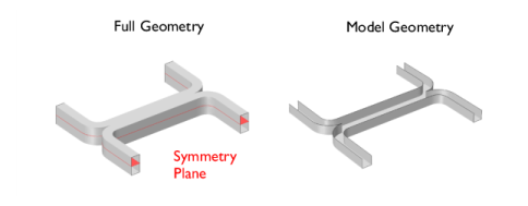
The geometry of the device is shown in Figure 5. The device geometry is split in two because of symmetry.