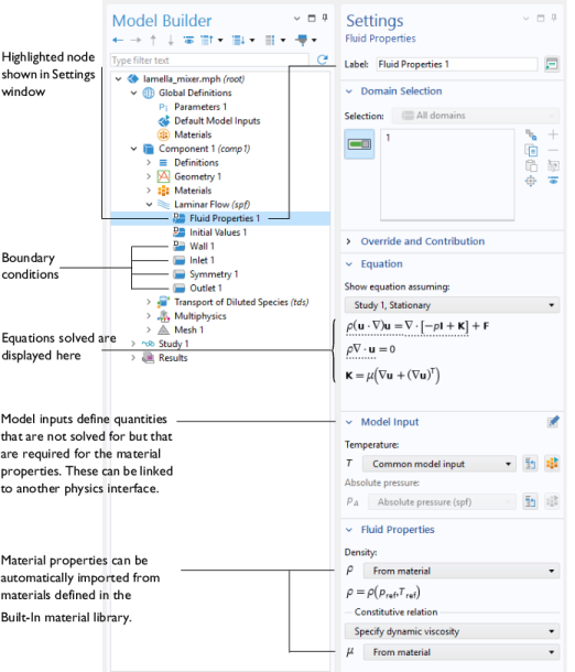
The Microfluidics physics interfaces are used to set up simulation problems. Each physics interface expresses the relevant physical phenomena in the form of sets of partial or ordinary differential equations, together with appropriate boundary and initial conditions. Each feature added to the physics interface represents a term or condition in the underlying equation set. These features are usually associated with a geometric entity within the model, such as a domain, boundary, edge (for 3D components), or point. Figure 1 uses the Lamella Mixer model (found in the Microfluidics Module application library) to show the Model Builder and the Settings window for the selected Fluid Properties 1 feature node. This node adds the Navier–Stokes equations to the simulation within the domains selected. Under the Fluid Properties section the settings indicate that the fluid density and viscosity are inherited from the material properties assigned to the domain. The material properties can be set up as functions of dependent variables in the model, for example, temperature and pressure. The wall, inlet, symmetry, and outlet boundary conditions are also highlighted in the model tree. The Wall boundary condition is applied by default to all surfaces in the model and adds a no-slip constraint to the flow. The inlet and outlet features include a range of options to allow fluid to enter or leave the simulation domain.

The Microfluidics Module includes a number of physics interfaces for modeling different types of microfluidic devices. When a new model is started, these physics interfaces are selected from the Model Wizard. Figure 2 shows the Model Wizard with the physics interfaces included with the Microfluidics Module. Also see Physics Interface Guide by Space Dimension and Study Type. Below, a brief overview of each of the Microfluidics Module physics interfaces is given.

Microfluidic flows usually occur at low Reynolds numbers. The Reynolds number (Re) is a measure of the ratio of the fluid viscous to the inertial forces acting on the fluid and is given by: Re = ρUL/μ, where ρ is the fluid density, U is a characteristic velocity, L is a characteristic length scale, and μ is the dynamic viscosity.

The Laminar Flow interface () applies when the Reynolds number is less than approximately 1000. The physics interface solves the Navier–Stokes equations, for incompressible, weakly compressible or compressible flows (for Ma<0.3, where Ma = U/c, and c is the velocity of sound in the fluid). This Fluid Flow interface also allows for the simulation of non-Newtonian flows.

The Two-Phase Flow, Level Set interface (), the Two-Phase Flow, Phase Field interface (), and the Two Phase Flow, Moving Mesh interface () are used to model two fluids separated by a fluid interface. The moving interface is tracked in detail using either the level set method, the phase field method, or by a moving mesh, respectively. The level set and phase field methods use a fixed mesh and solve additional equations to track the interface location. The moving mesh method solves the Navier–Stokes equations on a moving mesh with boundary conditions to represent the interface. In this case equations must be solved for the mesh deformation. Since a surface in the geometry is used to represent the interface between the two fluids in the Moving Mesh interface, the interface itself cannot break up into multiple disconnected surfaces. This means that the Moving Mesh interface cannot be applied to problems such as droplet formation in inkjet devices (in these applications the level set or phase field interfaces are appropriate). All three physics interfaces support both compressible (Mach number, Ma < 0.3) and incompressible laminar flows, where one or both fluids can be non-Newtonian. Two-Phase Flow, Level Set also supports porous domains.

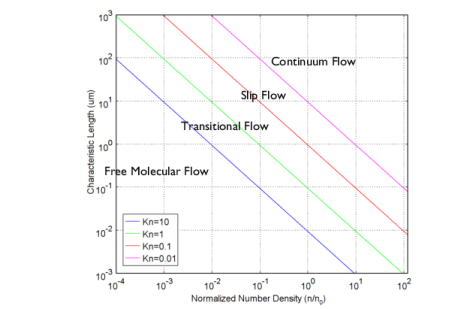
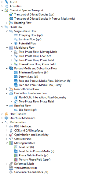
Rarefied gas flow occurs when the mean free path, λ, of the molecules becomes comparable with the length scale of the flow, L. The Knudsen number, Kn = λ/L, characterizes the importance of rarefaction effects on the flow. As the gas becomes rarefied (corresponding to increasing Knudsen number), the Knudsen layer, which is present within one mean free path of the wall, begins to have a significant effect on the flow. For Knudsen numbers below 0.01 rarefaction can be neglected, and the Navier Stokes equations can be solved with nonslip boundary conditions (the Laminar Flow () or Creeping Flow () interfaces can be used in this instance). For slightly rarefied gases (0.01 < Kn < 0.1), the Knudsen layer can be modeled by appropriate boundary conditions at the walls together with the continuum Navier–Stokes equations in the domain. In this instance the Slip Flow interface () is appropriate. To model higher Knudsen numbers the Molecular Flow Module is required. The figure below shows how high Knudsen numbers can be obtained either by reducing the size of the geometry, or by reducing the pressure or number density of the gas.