Microfluidic Devices: Physics and Applications
Microfluidic flows occur on length scales that are orders of magnitude smaller than macroscopic flows. Manipulation of fluids at the microscale has a number of advantages; typically microfluidic systems are smaller, operate faster, and require less fluid than their macroscopic equivalents. Energy inputs and outputs are also easier to control (for example, heat generated in a chemical reaction) because the surface-to-area volume ratio of the system is much greater than that of a macroscopic system.
In general, as the length scale (L) of the fluid flow is reduced, properties that scale with the surface area of the system become comparatively more important than those that scale with the volume of the flow. This is apparent in the fluid flow itself as the viscous forces, which are generated by shear over the isovelocity surfaces (scaling as L2), dominate over the inertial forces (which scale volumetrically as L3).
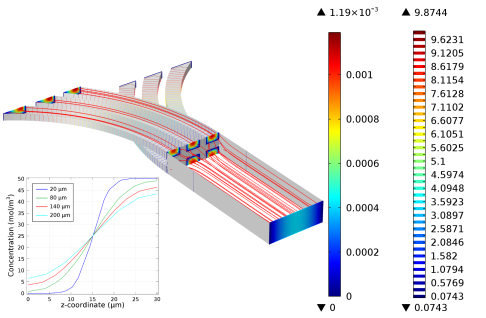
The Reynolds number (Re), which characterizes the ratio of these two forces, is typically low, so the flow is usually laminar (Re < 1000). In many cases the creeping (Stokes) flow regime applies (Re « 1). Laminar and creeping flows make mixing particularly difficult, so mass transport is often diffusion limited. The diffusion time scales as L2, but even in microfluidic systems diffusion is often a slow process. This has implications for chemical transport within microfluidic systems. The figure below shows flow in a device designed to enhance the mixing of two fluids in a lamella flow. Pressure contours are shown on the walls of the mixer, and the velocity magnitude is shown at the inlets and outlets of the mixer as well as at the point where the two sets of channels (carrying different fluids) converge. Streamlines (in red) are also plotted. The inset shows the concentration of a diffusing species present in only one of the fluids. It is plotted along vertical lines located progressively further down the center of the mixer.
When multiple phases are present, surface tension effects become important relative to gravity and inertia at small length scales. The Laplace pressure (the pressure jump across a two phase boundary), capillary force, and Marangoni forces all scale as 1/L. The figure below shows the break up of oil droplets to produce an emulsion as the oil flows into a channel carrying a second fluid. Velocity streamlines are shown and the fluid velocity is plotted on the symmetry plane. The two-phase boundary is shown in green.
Flow through porous media can also occur on microscale geometries. Because the permeability of a porous media scales as L2 (where L is the average pore radius) the flow is often friction dominated when the pore size is in the micron range and Darcy’s law can be used. For intermediate flows this module also provides a physics interface to model flows where the Brinkman equation is appropriate.
At the microscale, a range of electrohydrodynamic effects can be used to influence the fluid flow. The electric field strength for a given applied voltage scales as 1/L, making it easier to apply relatively large fields to the fluid with moderate voltages. In electroosmosis the uncompensated ions in the charged electric double layer (EDL) present on the fluid surfaces are moved by an electric field, causing a net fluid flow. Electrophoretic and dielectrophoretic forces on charged or polarized particles in the fluid can be used to induce particle motion, as can diamagnetic forces in the case of magnetophoresis. The manipulation of contact angles by the electrowetting phenomena is also easy in microscale devices, a phenomenon that has been used as a basis for various new display technologies. The figure below shows an adjustable focus liquid lens, whose radius of curvature can be adjusted using the electrowetting effect. The colors show the fluid velocity magnitude in a lower, oil-filled part of the lens and the arrow plot shows the velocity in the liquid above the oil lens.
As the length scale of the flow becomes comparable to intermolecular length scale, more complex kinetic effects become important. For gases, the ratio of the molecular mean free path to the flow geometry size is given by the Knudsen number (Kn). Clearly, Kn scales as 1/L. For Kn < 0.01, fluid flow is usually well described by the Navier–Stokes equations with no-slip boundary conditions. In the slip-flow regime (0.01 < Kn < 0.1), appropriate slip boundary conditions can be used with the Navier–Stokes equations to describe the flow away from the boundary. The Microfluidics Module includes a physics interface to deal with these slightly rarefied gas flows: the Slip Flow interface. For more highly rarefied flows, the Molecular Flow Module should be used.