For hypoeutectoid steels that are being cooled from an austenitic state, the phase transformations into different destination phases occur across certain temperature ranges. For example, no ferrite forms before the temperature falls below the Ae3 temperature in an Fe–C diagram, as austenite is stable above this temperature. Another example is the (eutectoid)
Ae1 temperature above which no pearlite forms. These temperatures, and other temperatures that are important when modeling phase transformations in steels, depend not only on the carbon content of the material, but also on other alloying elements. There exist several empirical models in the literature, and COMSOL Multiphysics provides several of these temperatures through the
Steel Composition node that can be used in the Metal Phase Transformation and Austenite Decomposition interfaces. The temperatures can be readily accessed by the
Phase Transformation nodes to facilitate phase transformation modeling.
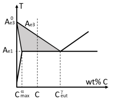
In an Fe–C diagram, the Ae1 and
Ae3 temperature lines represent the lower and upper limits of the two-phase ferrite–austenite region. For a steel of a given carbon content, the
Ae3 temperature can be viewed as a ferrite start temperature, that is, the upper temperature for ferrite formation when cooling the steel from the purely austenitic state. Similarly, the
Ae1 temperature can be viewed as the pearlite start temperature, see
Figure 3-5.
Andrews (Ref. 14) developed empirical models for these temperatures, based on the alloying elements of the material. The models are given by
where C,
Si,
Ni, and so forth, are the weight percentages of the respective alloying elements. These expressions are valid for steels with a carbon concentration less than 0.6% by weight. As an alternative to using the models by Andrews, you can use a parameterized description of the
Ae1 and
Ae3 temperature lines. To do this, you specify directly the
Ae3 temperature at zero carbon concentration,

, the
Ae1 temperature, and the eutectoid concentration of austenite,

. This gives the following linear expression for the
Ae3 temperature line:
where C is the carbon concentration of the steel. In contrast to the formulation by Andrews, the
Ae3 temperature line is here linear in the carbon concentration.
Unlike the Ae1 and
Ae3 temperatures, the onset of bainite formation does not correspond to an equilibrium temperature in the Fe–C diagram. Nevertheless, several empirical relationships for a bainite start temperature,
Bs, exist in the literature. COMSOL Multiphysics provides two models for this temperature. The model by Steven and Haynes (
Ref. 15) is given by