This phase transformation model is based on the work of Leblond and Devaux (Ref. 1). The model primarily considers carbon-diffusion-based phase transformations that occur in steels during heat treatment. Such transformations include austenite to ferrite, and austenite to bainite. There are four formulations for the Leblond–Devaux model:

where the phase transformation is active only when ; that is, when the right-hand side of Equation 3-3 is strictly positive. In general, the functions and are functions of temperature T. It was shown in Ref. 1 that the bainitic transformation additionally depends on the rate of cooling, . In this case, the functions and are functions of both T and .

where the phase transformation is active only when ; that is, when the right side of Equation 3-4 is strictly positive. The equilibrium phase fraction and the time constant are typically functions of temperature.

where is the initial phase fraction. This enables straightforward calibration of the model parameters from TTT diagram data. At a given temperature, and assuming that the initial phase fraction is zero, the equilibrium phase fraction of the destination phase is . A relative phase fraction of the destination phase is defined such that it is 1.0 as the equilibrium phase fraction is reached. The relative phase fraction X is given by

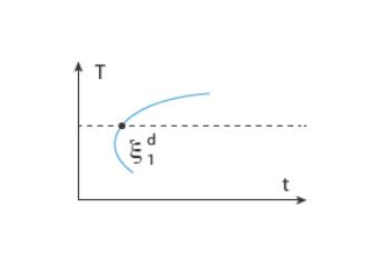
In the TTT diagram in Figure 3-1, a curve representing a fixed destination phase fraction is shown. At a fixed temperature T, this destination phase fraction is reached at time t1, so that

where t1 will vary with temperature, and the relative phase fraction X1 is understood to be the relative phase fraction corresponding to .

The Leblond–Devaux model can use a parameterized TTT diagram as input, in which a single TTT curve is used to identify the time constant. See Parameterized TTT Diagram.

This phase transformation model is based on the work by Leblond and others (Ref. 4).

In the equation above, the initial phase fraction is , and the equilibrium phase fraction , the time constant τs→d and the Avrami exponent ns→d are typically functions of temperature. On rate form, Equation 3-9 can be expressed as

where the explicit time dependence has been eliminated. The phase transformation is active only when ; that is, when the right side of Equation 3-10 is strictly positive. For the special case of ns→d = 1, the equation reduces to the time-and-equilibrium form of the Leblond–Devaux model (Equation 3-4). The JMAK phase transformation model in Equation 3-10 has a mathematical disadvantage in that an initial destination phase fraction equal to zero will yield a trivial zero solution, as the logarithm will evaluate to zero. There are different ways to circumvent this problem. One way is to require the initial phase fraction be assigned a small, but finite, value. Another way is to modify the rate equation itself, so that a zero initial phase fraction does not yield a trivial zero solution. In the phase transformation interfaces, the JMAK phase transformation model in Equation 3-10 is modified for phase fractions in the vicinity of . Below a certain threshold, the argument for the logarithm is modified so that the logarithm does not produce a zero value. This threshold phase fraction is set to 10-5 by default. A problem can arise in the case of nonzero initial phase fractions. Namely, if other phase transformations in the model operate such that the metallurgical phase that is the destination phase fraction above decreases, the JMAK model would run into problems as , whereby the argument in the logarithm becomes negative. One way to handle this is to exclude the effect of the initial phase fraction in the rate expression in Equation 3-10. This is done in COMSOL Multiphysics. A judgment has to be made in each situation whether this is a proper modeling assumption.

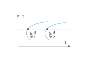
As in the case of the Leblond–Devaux model, the JMAK model can be calibrated using TTT diagram data. The integrated form in Equation 3-9 is used to calibrate the time constant τs→d and the Avrami exponent ns→d. To calibrate these two phase transformation model parameters, two curves are needed from a TTT diagram; see Figure 3-2. As for the Leblond–Devaux model, a zero initial phase fraction is assumed when calibrating the JMAK model. At a fixed temperature T, the two destination phase fractions are reached at times t1 and t2, respectively, so that

where the relative phase fractions X1 and X2 are understood to be the relative phase fractions corresponding to and , respectively. The transformation times t1 and t2 will vary with temperature.

The JMAK model can use a parameterized TTT diagram as input, in which two TTT curves are used to identify the time constant and the Avrami exponent. See Parameterized TTT Diagram.

The JMAK model can use a parameterized TTT diagram as input, in which a single TTT curve is used to identify the time constant. Using this formulation, you specify the Avrami exponent separately. See Parameterized TTT Diagram.

This phase transformation model is based on the work by Kirkaldy and Venugopalan (Ref. 11), and extended and modified by several others. There are three formulations for the Kirkaldy–Venugopalan, simplified phase transformation model:

where is the equilibrium phase fraction, is a reference rate that in principle depends on temperature, chemical composition, and grain size, and Cr is a retardation coefficient. The relative phase fraction X is defined as

so that the rate of formation of the destination phase approaches zero as the relative phase fraction approaches one; that is, when the phase transformation nears completion. The Kirkaldy–Venugopalan, simplified phase transformation model shares the mathematical disadvantage with the JMAK model in that an initial destination phase fraction of zero will yield a trivial zero solution. Similar to the JMAK phase transformation model, the Kirkaldy–Venugopalan, simplified phase transformation model is modified. A small threshold value for the destination phase fraction ξd is introduced, so that the phase transformation model produces a nonzero rate below this value.

The Kirkaldy–Venugopalan, simplified phase transformation model can be calibrated using TTT diagram data. Similar to the cases of the Leblond–Devaux and JMAK phase transformation models, the expression for the rate of destination phase formation is used to identify the model parameters, here the rate coefficient . Rearranging the rate expression in Equation 3-15 gives an expression of the form

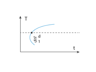
where the relative phase fraction X has been used. Note that at a fixed temperature, the equilibrium phase fraction is constant, and it can therefore be included in the rate term in Equation 3-17. The reference rate is temperature dependent (and dependent on chemical composition and grain size, in the original Kirkaldy–Venugopalan formulation. (See The Microstructure Based Model). At a fixed temperature, t1 is the time to reach the destination phase fraction (or alternatively, to reach the relative phase fraction X1), see Figure 3-3. This is expressed as

Using Equation 3-17, the rate coefficient is expressed as

Note that if the retardation coefficient Cr is known, the integral can be computed a priori for a fixed X1. The rate coefficient is therefore inversely proportional to the time it takes to reach the relative phase fraction X1. The time t1 generally depends on temperature.

The Kirkaldy–Venugopalan, simplified model can use a parameterized TTT diagram as input, in which a single TTT curve is used to identify the rate coefficient. See Parameterized TTT Diagram.

where is the equilibrium phase fraction, fG is a function of the ASTM grain size, fC is a function of chemical composition, and fT is an Arrhenius term. The rate depends on the level of undercooling |Tu − T| below an upper temperature limit Tu. The exponent m is an undercooling exponent. The exponent a in the rate term that alters the characteristic of the sigmoid function. The phase transformation is accompanied by the definition of a lower temperature limit Tl, below which the transformation becomes inactive. The term Cr is a retardation coefficient. The functions (grain size dependence, chemical composition dependence, and the Arrhenius term) are collected into a single function f = fG fC fT, which, together with the undercooling term, can be interpreted as the reference rate of the Kirkaldy–Venugopalan, simplified model. Note that the rate equation is dimensionally incorrect in its original formulation by Kirkaldy and Venugopalan. The equation is taken as is, with the understanding that temperature unit is Kelvin, and the resulting rate unit is one per second. The relative phase fraction X is defined as

so that the rate of formation of the destination phase approaches zero as the relative phase fraction approaches one; that is, when the phase transformation nears completion. The sigmoid function used in the Microstructure based phase transformation model has mathematical disadvantages that it shares with the Kirkaldy–Venugopalan, simplified phase transformation model, see The Kirkaldy–Venugopalan, Simplified Model.

This phase transformation model was developed by Koistinen and Marburger (Ref. 2) to model the diffusionless (displacive) austenite to martensite transformation in iron-carbon alloys and carbon steels. The onset of the transformation, which only occurs on cooling, is characterized by a critical start temperature — the martensite start temperature Ms. Above this temperature, no transformation from austenite (the source phase) to martensite (the destination phase) occurs. Below Ms, the amount of formed martensite is proportional to the undercooling below Ms, given by Ms − T. On rate form, the Koistinen–Marburger equation can be written

where β is the Koistinen–Marburger coefficient. Note that the transformation of austenite into martensite only occurs below Ms and only during cooling (that is, when ). To make the onset of martensitic transformation numerically smooth, a parameter ΔMs is used. The smoothing parameter defines a smoothed Heaviside function that makes the onset of martensitic transformation gradual. The parameter should be chosen small enough that the start temperature characteristic is retained. Assuming a constant cooling rate and that the phase fraction of austenite at Ms is , the rate equation can be integrated to

This integrated form is commonly found in the literature. Instead of defining the Koistinen–Marburger coefficient directly, a martensite finish temperature, M90, can be defined, corresponding to reaching a phase fraction of 90% using Equation 3-24, and assuming 100% initial source phase fraction. The Koistinen–Marburger coefficient β is then given by

The rate form of Equation 3-23 is more general, and from a computational standpoint it is more suitable for implementation. The rate form is therefore used in the phase transformation interfaces.

It has been recognized that the onset of martensitic transformation can be affected by an externally applied stress. The martensite start temperature is commonly shifted by a linear combination of the externally applied hydrostatic stress and the externally applied von Mises effective stress. In Ref. 3 the shift in martensite temperature is expressed as

where we have used the coefficient names a1 and a2, and the pressure instead of the hydrostatic stress.

This phase transformation model can be used for example to model dissolution of α phase in titanium, on heating. It is based on the idea that the rate of formation of a phase is inversely proportional to its phase fraction. Here, it is expressed as

In this phase transformation model, the “equilibrium phase fraction” does not represent a true equilibrium phase fraction in the sense that the phase transformation would saturate to this value. Nevertheless, it is used as a parameter in the definition of X, for consistency. By combining the previous two equations, the rate equation used in COMSOL Multiphysics becomes

for . For isothermal or cooling conditions, the rate is zero. Integrating the rate equation in Equation 3-28, and using the fact that the destination phase begins to form only once the lower temperature limit Tl is reached, the following linear expression is obtained for the evolution of the destination phase fraction with temperature.

This phase transformation model was originally developed to model the dissolution of pearlite and the formation of eutectoid austenite during heating of hypoeutectoid steels. Its rate equation is of the same form as the Johnson–Mehl–Avrami–Kolmogorov phase transformation model (Equation 3-10), and it is given by

and the Avrami constant, according to Oddy and others (Ref. 20) is set to ns → d = 3, and the time parameters are given by

Using this option, other types of phase transformations can be defined. A user-defined phase transformation assumes that a source phase decomposes into a destination phase according to Equation 3-1.