Calibration of Phase Transformation Models
During a thermal transient, a material point may undergo varying rates of cooling and heating. During this transient, several phase transformations can be active at the same time. This suggests that it is difficult to calibrate phase transformation models individually, as they tend to affect one another. For example, in the case of austenite decomposition, it is common in practice to present the complicated nature of phase transformations as continuous cooling transformation (CCT) or time-temperature transformation (TTT) diagrams; see Figure 2-1 and Figure 2-2 for schematic examples. Both diagrams show the start temperatures for the formation of a small fraction of different phases (Fs for the start temperature of ferrite, and so on). The fraction can be chosen arbitrarily but is often 0.1% or 1%. The difference between the two diagram types, as their names imply, is the following:
One method to measure the actual start temperatures required to draw each diagram is to use dilatometry experiments. Metallurgical phase transformations are accompanied by a change in volume, owing to the density difference between phases. In a dilatometer, a specimen is cooled (or heated), and its length is monitored. The specimen length will change according to basic thermal expansion, but phase transformations will induce additional length changes that can be measured.
In a real quenching situation, it is clear that material points do not experience either of the two extremes represented by the CCT and TTT diagrams (constant temperature rate versus constant temperature). Nevertheless, because experimentally obtained CCT and TTT diagrams are very common in the heat treatment community, phase transformation models must in practice be calibrated using them.
It is here useful to examine one formulation of the Leblond–Devaux model:
In this equation, the phase fraction for the destination phase tends toward an equilibrium value , and the rate at which this occurs is characterized by the time constant τs → d. Note here that the equilibrium phase fraction and the time constant are in general both temperature dependent, and that temperature in turn varies with time. At constant temperature, the equation can be integrated analytically, giving
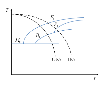
The equilibrium phase fraction can be deduced from an (equilibrium) iron–carbon diagram (Ref. 1) or from dilatometry experiments at a very low temperature rate (or at constant temperature after a rapid temperature drop). If we know this equilibrium phase fraction at a given temperature 
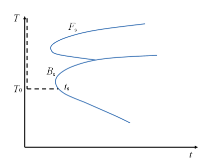
t1, we can compute the temperature-dependent time constant from knowing the time it takes to reach a specific phase fraction (isothermally):
Alternatively, if we know the time to reach, for example, 1% of the equilibrium phase fraction, that is, the relative phase fraction
the time constant is obtained without knowing the equilibrium phase fraction. Thus, a TTT diagram showing curves of transformation times corresponding to relative phase fractions X can straightforwardly be used to compute the temperature-dependent time constant. In this sense, a TTT diagram is easier to use for phase transformation model calibration than a CCT diagram. This method to the calibration of phase transformation models to TTT diagram data can be used also for the Johnson–Mehl–Avrami–Kolmogorov (JMAK) and Kirkaldy–Venugopalan models. It should be pointed out that given a set of phase transformation model parameters, it is straightforward to compute both types of diagrams and to adjust the model parameters based on comparisons of the computed diagrams and experimental information. It is sometimes necessary to iterate in this manner to find a sufficiently accurate set of model parameters.
As a final alternative to performing the calibration using TTT or CCT diagrams, you can import computed phase transformation data. This is described in Importing Material Properties and Phase Transformation Data.
Figure 2-1: A CCT diagram showing how phases appear during cooling at two different rates. The temperatures corresponding to 1% formed fraction of ferrite, pearlite, and bainite are shown. The martensite start temperature is shown as a straight line. The time is shown on a logarithmic axis.
Figure 2-2: A TTT diagram showing how the temperature is rapidly decreased to a fixed value T0 and then kept constant.
For an example how to compute CCT and TTT diagrams, see Transformation Diagram Computation: Application Library path Metal_Processing_Module/Transformation_Diagrams/transformation_diagram_computation.
For an example how to calibrate a phase transformation model based on experimental TTT diagram data, see Transformation Diagram Computation: Application Library path Metal_Processing_Module/Transformation_Diagrams/calibration_against_ttt_data.