COMSOL 6.4 - Results

In the Model Builder window, under Results

Much of the structure has essentially zero movement in this initial study. To facilitate results analysis, add a selection to the solution, so that only the domains of interest are displayed in the plots.

Datasets

In the Model Builder window, expand the Results > Datasets node

, then click Study 1/Solution 1 (sol1)

Selection

In the Results toolbar, click Attributes

and choose Selection

In the Settings window for Selection, locate the Geometric Entity Selection section. From the Geometric entity level list, choose Domain.

From the Selection list, choose Electrostatics.

Select the Propagate to lower dimensions checkbox.

Displacement (solid)

In the Model Builder tree click the Displacement (solid)

node.

Click the Zoom Extents button

at the top of the Graphics window.

The plot now shows the displacement of the diaphragm only, which, as expected, is maximum in the center of the sensor.

Next, plot the electric potential in an xy-oriented plane between the sensor diaphragm and the ground plane.

Electric Potential (es)

In the Model Builder window, expand the Results > Electric Potential (es) node

, then click Multislice 1

In the Settings window for Multislice, locate the Multiplane Data section.

Find the x-planes subsection. In the Planes text field, type 0.

Find the y-planes subsection. In the Planes text field, type 0.

Find the z-planes subsection. From the Entry method list, choose Coordinates.

In the Coordinates text field, type -0.0023[mm].

Click to expand the Range section. Select the Manual color range checkbox.

In the Minimum text field, type 0.

In the Maximum text field, type 1.

Selection 1

Right-click Results > Electric Potential (es) > Multislice 1

and choose Selection

In the Settings window for Selection, locate the Selection section. From the Selection list, choose Cavity.

On the Electric Potential (es) toolbar, click the Plot button

Due to the deformation of the diaphragm the potential is nonuniformly distributed in the plane, which cuts through the cavity at a constant height.

Next, the deformation of the diaphragm is plotted as a function of the pressure difference across it. Both the average and the maximum displacements are plotted.

1D Plot Group 5

In the Home toolbar click Add Plot Group

and choose 1D Plot Group

On the 1D Plot Group 5 toolbar click Global

Global 1

Use the point integration and surface average operators defined earlier to evaluate the displacement at the midpoint of the membrane and the average displacement.

In the Settings window for Global locate the y-Axis Data section. In the table, enter the following settings:


Expression	Unit	Description
intop1(w)	um	Maximum Displacement
aveop1(w)	um	Average Displacement

1D Plot Group 5

In the Model Builder window click 1D Plot Group 5

In the Settings window for 1D Plot Group 5, click to expand the Title section.

From the Title type list, choose Manual.

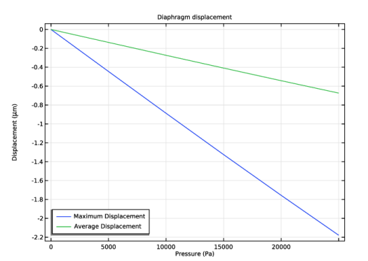
In the Title text field, enter Diaphragm Displacement.

Locate the Plot Settings section.

Select the x-axis label checkbox. In the x-axis label text field, enter Pressure (Pa).

Select the y-axis label checkbox. In the y-axis label text field, enter Displacement (\mu m).

Click to expand the Legend section. From the Position list, choose Lower left.

In the Label text field enter Diaphragm Displacement vs Pressure.

On the Diaphragm Displacement vs Pressure toolbar, click Plot

At an applied pressure of 10 kPa the diaphragm displacement in the center is 0.89 μm. The average displacement of the diaphragm is 0.27 μm. These values are in good agreement with the approximate model given in Practical MEMS (maximum displacement 0.93 μm, average displacement 0.27 μm).

Now plot the sensor capacitance as a function of the applied pressure. If the switched capacitor amplifier described in Practical MEMS is used to produce the output, the sensor output or transfer function is directly proportional to the change in capacitance.

1D Plot Group 6

In the Home toolbar, click Add Plot Group

and choose 1D Plot Group

On the 1D Plot Group 6 toolbar click Global

Since the terminal boundary condition was used for the underside of the diaphragm, COMSOL Multiphysics automatically computes its capacitance with respect to ground. The value of the capacitance is available as a variable in result analysis.

In the Settings window for Global, click Replace Expression

in the upper-right corner of the y-Axis Data section. From the menu, navigate to Component 1 > Electrostatics > Terminals > es.C11 - Maxwell capacitance - F; then double click to choose the item.

Next, compare the computed capacitance with the small displacement, linearized analytic expression derived in Practical MEMS.

Locate the y-Axis Data section. In the table, change the unit of the first row to pF and enter the second row, as shown below:


Expression	Unit	Description
es.C11	pF	Capacitance
0.738[pF](1+8.87e-6[1/Pa]p0)	pF	Linearized Analytic Capacitance

In the Model Builder window click 1D Plot Group 6

In the Settings window for 1D Plot Group locate the Title section.

From the Title type list, choose Manual.

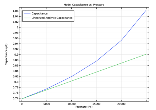
In the Title text area, enter Model Capacitance vs Pressure.

Locate the Plot Settings section.

Select the x-axis label checkbox. In the x-axis label text field, enter Pressure (Pa).

Select the y-axis label checkbox. In the y-axis label text field, enter Capacitance (pF).

Locate the Legend section. From the Position list, choose Upper left.

In the Label text field enter Model Capacitance vs Pressure.

Click Plot

The capacitance of the sensor increases with applied pressure. The gradient of the curve plotted gives a useful measure of the response of the device. At the origin the response of the model (1/4 of the whole sensor) is 7.3×10-6 pF/Pa, compared to the simple analytical response of 6.5×10-6 pF/Pa. The response for the whole sensor is therefore 29×10-6 pF/Pa compared to the analytic value of 26×10-6 pF/Pa. With the measurement circuit proposed in Practical MEMS this corresponds to a sensor transfer function of 29 μV/Pa for the COMSOL Multiphysics model and 26 μV/Pa for the simple analytic model. The response is nonlinear, so that at 20 kPa the model output is 14×10-6 pF/Pa (device output 57 pF/Pa).

Next, add thermal expansion to the model, to assess the effects of packaging stresses on the device performance.