COMSOL 6.4 - The Joints Interface

The interface (

), found under the branch (

) when adding a physics interface, is intended for analysis of mechanical assemblies. The parts in the assembly can be rigid or flexible, and are connected by various types of joints. Flexible parts can be defined using solid, shell, or beam elements. Different structural elements can be connected through joints by defining nodes on the boundaries of solid element, edges of a shell element, or points on the beam element. With the Nonlinear Structural Materials Module, you can also incorporate nonlinear material models like hyperelasticity or plasticity by adding a Solid Mechanics interface to the model.

There are many types of joints, such as hinges or ball joints, which can be used based on the type of connection required between components. The joints can be given properties such as spring constants, damping, friction, and limits on movement. The computed results are relative displacements, rotations, angular velocities, accelerations, and forces.

To connect various components, you add joint nodes to the model either through a Multibody Dynamics interface or a Joints interface. The Multibody Dynamics interface is ideal for true multibody problems that involve analyzing dynamics of interacting components. In contrast, the Joints interface is suitable for cases that do not involve actual multibody dynamics, but still require joints. In such cases, using the Joints interface simplifies and streamlines the workflow for connecting multiple structural components.

The is the default physics interface name.

The is used primarily as a scope prefix for variables defined by the physics interface. Refer to such physics interface variables in expressions using the pattern <name>.<variable_name>. In order to distinguish between variables belonging to different physics interfaces, the name string must be unique. Only letters, numbers, and underscores (_) are permitted in the field. The first character must be a letter.

The default (for the first physics interface in the model) is joints.

From the list, select or . Use to treat the mechanical behavior as quasi static (with no mass effects, that is, no second-order time derivatives). Selecting this option gives a more efficient solution for problems where the variation in time is slow when compared to the natural frequencies of the system.

This is an information table that displays the name of all the joints used in a model and their source and destination attachments. This table summarizes all the connections present in a model and can be used to review the connections.

This is an information table that displays the number of degrees of freedom and constraints introduced by joints. You can use this information to determine whether you model has an appropriate number of constraints or not when running pure rigid body analysis.

The contents of the columns are:

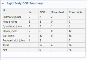
The last two rows of the table contain a summary. In the row, the number of DOFs, prescribed conditions, and constraints are summed.

The row contains the net number of degrees of freedom of the model — that is, the difference between all degrees of freedom and the constraints and prescribed motions. A negative net number of degrees of freedom indicates that the mechanism is overconstrained and is not shown. In that case, the net number of constraints is instead displayed.

Some constraints are conditional and are not present during the whole analysis. Such constraints are counted in the summary table, irrespective of their actual status.

The contents of the table do not change if you suppress any of the contributing features from the settings in the study step.

In general, and if there are flexible bodies in the system, the total number of degrees of freedom increase significantly. Such degrees of freedom are not accounted for in the summary.

To display this section, click the button (

) and select in the dialog. Normally these settings do not need to be changed.

You can choose how extra ODE variables added by joints are grouped in the node of a generated solver sequence.

The selection made in this section can be overridden by the settings in the section of the individual joint nodes.

To display the contents of this section, click the button (

) and select in the dialog. Normally these settings do not need to be changed.

From the , you can specify the value type () of dependent variables when the setting is activated in the node of any solver sequence used.

Each joint adds a number of global dependent variables depending on the number of ODEs needed to represent its motion. The displacement ODE variables in all joints are grouped in a single ODE entity. Similarly, rotational ODE variables in all joints are grouped in another single ODE entity. The default name of displacement and rotational collection for the first physics interface in the model are joints_disp and joints_rot. Subsequently added interfaces automatically get the first unique name. The name can be changed, but a field name must not coincide with the name of a field of another type, or with a component name belonging to some other field. Component names must be unique within a model.