Extracting Reduced-Order State-Space Matrices
The tutorial in this section illustrates how to use the mphreduction function to extract the state-space matrices for a model. The studied heat transfer model contains a heat source, which is set as input in the state-space system. The temperature at a specific point is used as output. Follow the step-by-step instructions below to obtain the state-space matrices and to solve the system in Simulink.
Model Definition in the COMSOL Desktop
1
2
In the File menu, select Application Libraries.
3
In the Application Libraries, browse to LiveLink for Simulink > Tutorials, and select model_tutorial_llmatlab. Click Open.
Model Parameters
The loaded model is used as base model for documentation tutorial. The geometry, mesh, and physics is set, but for this specific problem you need to edit the model to use parameters for the initial and external temperature as they will be used later in the reduced model.
1
Under Global Definitions, select Parameters 1 node.
2
In the Settings window for Parameters, update the table according to the settings below:
Physics Settings — Heat Transfer in Solids
In this section you will set up the Heat Transfer in Solids physics interface. If you do not have the Heat Transfer Module or MEMS Module skip the instructions below and go directly to Physics Settings — General Form PDE.
1
In the Model Builder, select Heat Transfer in Solids > Initial Values 1 node. In the Settings window set the Temperature field to T0.
2
In the Model Builder, select Heat Transfer in Solids > Heat flux 1 node. In the Settings window enter Text in External temperature field.
Even though you can generate ROM including constraint models in COMSOL, the resulting reduced matrices are not suited for Simulink state-space system. In this model the bottom temperature is imposed as a constraint, you will change it to heat flux condition instead.
3
Right-click Heat Transfer in Solids > Temperature 1 node, and select Disable.
4
Right-click Heat Transfer in Solids node, and select Heat Flux.
5
6
Under Heat Flux, select Convective heat flux.
7
In the Heat transfer coefficient field enter 1e6.
8
In the External temperature field enter Temp.
You have now set up the physics, and can go directly to Study Settings to continue.
Physics Settings — General Form PDE
In this section you will find the instruction to set up the physics using the General Form PDE interface. If you have the Heat Transfer Module or MEMS Module skip the instructions in this section and go directly to Study Settings.
1
In the Model Builder, right-click Heat Transfer in Solids node and select Disable.
2
In the Physics toolbar select Add Physics.
3
In the Add Physics window, expand Mathematics > PDE Interfaces. Select General Form PDE (g) and click Add to Component 1.
4
In the Settings window for General Form PDE, under Units section click Select Dependent Variable Quantity.
5
In the Physical Quantity window, expand General, and select Temperature (K). Click OK.
6
In the Settings window for General Form PDE, under Units section click Select Source Term Quantity.
7
In the Physical Quantity window, expand Transport, and select Heat source (W/m^3). Click OK.
8
In the Model Builder, expand General Form PDE and select General Form PDE 1 node.
9
In the Settings window for General Form PDE, under Conservative Flux section in the Γ table enter:
10
In the Settings window for General Form PDE, under Source Term section in the f text field enter 0.
11
In the Settings window for General Form PDE, under Source Term section in the da text field enter material.rho*material.Cp.
12
In the Model Builder, expand General Form PDE and select Initial Values 1 node.
13
In the Settings window for Initial Values, under Initial Values section in the Initial value for u field enter T0.
14
In the Model Builder, right-click General Form PDE and select Source.
15
In the Settings window for Source, select domain 2.
16
In the Settings window for Source, in the Source Term field enter power/(1[cm]*1[cm]*1[mm]).
17
In the Model Builder, right-click General Form PDE and select Flux/Source.
18
In the Settings window for Flux/Source, select boundaries 7 8 10 11 12.
19
In the Settings window for Flux/Source, in the Boundary Flux/Source field enter 10[W/(m^2*K)]*(Text-u).
20
In the Model Builder, right-click General Form PDE and select Flux/Source.
21
In the Settings window for Flux/Source, select boundaries 3.
22
In the Settings window for Flux/Source, in the Boundary Flux/Source field enter 1e6[W/(m^2*K)]*(Temp-u).
Study Settings
To create a reduced-order model, first add an unreduced model study and a training study to your model. In this section you will add a Time Dependent study and an eigenfrequency study that will be later be set as unreduced model and training studies, respectively.
1
In the Study toolbar, select Add Study.
2
In the Add Study window, select Time Dependent and click Add Study.
3
In the Settings window for Time Dependent, enter range(0,1,50) in the Output times field.
Add a domain point probe plot, which will define the output of the reduced-order model.
4
Under Component 1 node, right-click Definitions and select Probes > Domain Point Probe.
5
In the Settings window for Domain Point Probe, locate the Coordinates field and enter: 1e-2 1e-2 1e-2.
6
In the Study toolbar, select Compute.
7
In the Add Study window, expand More Studies and select Eigenvalue. Then click Add Study.
8
In the Settings window for Eigenvalue, select Desired number of eigenvalues and enter 60.
9
In the Settings window for Eigenvalue, select Search for eigenvalues around and leave it with the default value.
10
In the Study toolbar, select Compute.
Reduced-Order Model
Before adding a reduced-order study to your model you need to set the input, define the power variable power, the bottom temperature Temp, and the exterior temperature Text.
1
In the Model Builder, click Show More Options.
2
In the Show More Options window, under Study, select Reduced-Order Modeling.
3
Right-click Global Definitions and select Reduced-Order Modeling > Global Reduced Model Inputs.
4
In the Settings window for Global Reduced Model Inputs, edit the table as defined below:
In the step below you will now add a model reduction study.
5
In the Add Study window, select Empty Study, and click Add Study.
6
Right-click Study 3, and select Model Reduction.
7
In the Settings window for Model Reduction, under Model Reduction Settings section enter the following settings:
8
Under the Outputs section, enter the table as defined below:
9
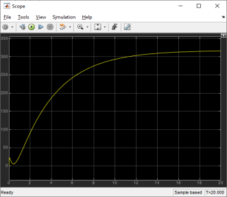
Now click Compute to generate the reduced-order model.
10
Extracting the State Space Matrices in MATLAB
1
model = mphload(<modelname>);
where <modelname> is the name of the Model MPH file. If the model file path is not set in MATLAB you can enter the full path of the model name.
2
A call to mphreduction creates the state-space matrices needed to simulate the reduced-order system. Enter:
M = mphreduction(model, 'rom1')
3
power = 30;
Temp = 300;
Text = 300;
Run the Simulation in Simulink
1
At the MATLAB prompt, enter simulink to start Simulink.
2
In the Simulink Start Page window, select Blank Model.
3
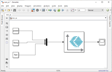
From the Simulink Library Browser drag the COMSOL Reduced Order SS block from the COMSOL 6.4 library into the empty Simulink diagram.
4
Double-click the COMSOL Reduced Order SS block and make sure that the System variable name is M
5
Continue editing the Simulink diagram by adding constant block, a MUX block and a scope so it looks like in the figure below:
6
In the Simulation toolbar, locate Simulation stop time and enter 20.
7