where ftag is the curve interpolation node and <data> can either be a 2-by-N cell array or a 2-by-N array.

where type can either be 'solid' to generate a solid object, 'closed' to generate a closed curve or 'open' to generate an open curve.

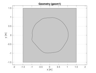
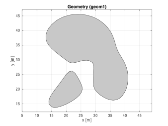
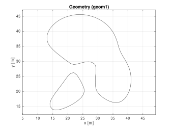
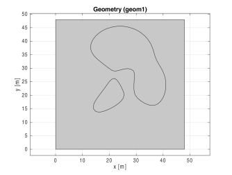
Use the function mphimage2geom to create geometry from image data. The image data format can be M-by-N array for a grayscale image or M-by-N-by-3 array for a true color image. This section also includes an example (see Example: Convert Image Data to Geometry).

If you specify the image data and the level value that represents the geometry contour you want to extract, the function mphimage2geom returns a model object with the desired geometry:

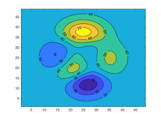
where imagedata is a C array containing the image data, and level is the contour level value used to generate the geometry contour.

where type is 'solid' and generates a solid object, 'closed' generates a closed curve object, or 'open' generates an open curve geometry object.

Use the property curvetype to specify the type of curve used to generate the geometry object:

where curvetype can be set to 'polygon' to use a polygon curve. The default curve type creates a geometry with the best suited geometrical primitives. For interior curves it uses interpolation curves, while for curves that are touching the perimeter of the image a polygon curve is used.

To scale the geometry use the scale property where scale is a double value:

Set the minimum distance (in pixels) between coordinates in curve with the mindist property where mindist is a double value:

Set the minimum area (in square pixels) for interior curves where minarea is a double value:

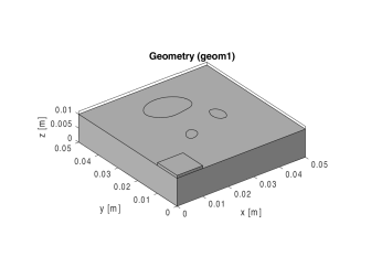
In case of overlapping solids, the function mphimage2geom automatically creates a Compose node in the model object. If you do not want this geometry feature, set the property compose to off:

To create a rectangle domain surrounding the object generated use the property rectangle:

 mphimage2geom returns a model object with the created geometry stored in a geometry node. The default geometry node has the tag geom1, to specify manually the geometry tag use the function as below:

where <geomtag> is a string corresponding to the tag of the geometry node.

where <geomnode> is the geometry node object where to include the newly generated geometry.

To manually specify the tag of the model object created in the COMSOL server use the command below:

where <Modeltag> is a string defining the tag of the model object in the COMSOL server.

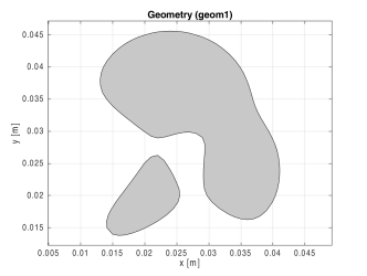
Use the property type to create closed or open curves. For example, to create a geometry following contour 40 with closed curves, enter:

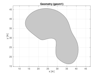
To scale the geometry, use the scale property. Using the current model scale the geometry with a factor of 0.001 (1e-3):

To insert a rectangle in the geometry that has an outer domain surrounding the created contour, set the property rectangle to on: