Use state-space export to create a linearized state-space model corresponding to a COMSOL Multiphysics model. You can export the matrices of the state-space form directly to the MATLAB® workspace with the command mphstate.

This section includes information about The State-Space System, how to Extract State-Space Matrices and Set Linearization Points and has an Extracting State-Space Matrices.

where x is the state variable vector.

If the components of the mass matrix MC are small, it is possible to approximate the dynamic state-space model with a static model, where :

Let Null be the PDE constraint null-space matrix and ud a particular solution fulfilling the constraints. The solution vector U for the PDE problem can then be written

where u0 is the linearization point, which is the solution stored in the sequence once the state-space export feature is run.

The input parameters should contain all parameters that are of interest as input to the model. Moreover, if you have any settings in a model that are connected to the degrees of freedom, like a constraint condition or a spring condition. These have to be declared as input in your state-space system. When solving the state-space system in MATLAB, subtract to these inputs the initial value of the corresponding DOF, as it is done in the example Extracting State-Space Matrices.

The function mphstate requires that the input variables, output variables, and the list of the matrices to extract in the MATLAB workspace are all defined:

where <soltag> is the solver node tag used to assemble the system matrices listed in the cell array out, and <input> and <output> are cell arrays containing the list of the input and output variables, respectively.

The output data str returned by mphstate is a MATLAB structure and the fields correspond to the assembled system matrices.

The system matrices that can be extracted with mphstate are listed in the table:

To extract sparse matrices set the property sparse to on:

To keep the state-space feature node, set the property keepfeature to on:

mphstate uses linearization points to assemble the state-space matrices. The default linearization point is the current solution provided by the solver node, to which the state-space feature node is associated. If there is no solver associated to the solver configuration, a null solution vector is used as a linearization point unless you manually set the linearization point to an existing solution.

You can manually select the linearization point to use. Use the initmethod property to select a linearization point:

where method corresponds to the type of linearization point — the initial value expression ('init') or a solution ('sol').

To set the solution to use for the linearization point, use the property initsol:

where <initsoltag> is the solver tag to use for a linearization point. You can also set the initsol property to 'zero', which corresponds to using a null solution vector as a linearization point. The default is the current solver node where the assemble node is associated.

For continuation, time-dependent, or eigenvalue analyses you can set which solution number to use as a linearization point. Use the solnum property:

where <solnum> is an integer value corresponding to the solution number. The default value is the last solution number available with the current solver configuration.

If there is a solver associated to the solver configuration <soltag>, you need to extract the matrices after the Dependent Variables node in the solver configuration, to proceed use the property extractafter as in the command below:

where <vtag> is the tag of the Dependent Variable node.

State-space models can be defined using the ss and sparss functions. The sparss function can be used if the state-space matrices are sparse. The system can be simulated using the lsim function. In order to create a reduced-order system using MATLAB, you can use the balred function. This function only accepts the use of full matrices. Hence, the function ss is used for defining the state-space system in MATLAB. Note that calling the function ss with argument matrices that are sparse results in a set of warnings. These warnings can be ignored.

The code below show how to use the Control System Toolbox to solve a dynamic system from the A, B, C, and D matrices obtained using mphstate:

where <input> is the input vector of the state space system, and <tspan> is the time step list.

You can obtain a reduced-order model using the balred function.

where <order> is the desired order reduction, and <tfinal> the simulation end time.

In this section you will find an example that illustrates how to use the mphstate function to extract the state-space matrices.

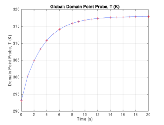
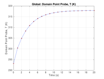
This is the same problem solved as in Extracting Reduced-Order State-Space Matrices, so you can compare the solution and computational performance when solving the problem with reduced-order model state-space system matrices.

First, load the model model_tutorial_llmatlab from the Application Library:

Extract the state-space system matrices Mc, MA, MB, C, and D of the model, with power, Temp, and Text as inputs and the probe evaluation comp1.ppb1 as the output:

The state-space formulation that uses the mass matrix is prepared to use sparse matrices and can often be simulated much faster. In order to simulate systems that involve a mass matrix on the left-hand side, you must switch to one of the simulation functions that support a mass matrix. Such MATLAB functions are ode15s, ode23s, and ode23t. ode15s and ode23t can solve problems with a singular mass matrix. Compute the state-space system with the extracted matrices,

Compare the solution computed with the system and the one computed with COMSOL Multiphysics (see Figure 4-1):

For some types of control system design, the use of the matrices A, B, C, and D are commonly used. Extract the state-space system matrices A, B, C, and D of the model with power, Temp, and Text as inputs and the probe evaluation comp1.ppb1 as the output:

Compare the solution computed with the previous system (see Figure 4-2):