Computing and Plotting the Results
Once the model is set up, the solution can be computed. A default mesh is automatically generated.
1
In the Study tab in the ribbon, click Compute
.
2
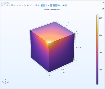
Click the Temperature (ht) node to display the temperature field at the geometry surface.
3
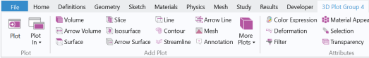
Visualize the material thermal conductivity on the geometry by adding a new 3D Plot group. In the Results tab, select 3D Plot Group
. An additional tab containing Plot Tools for the 3D Plot Group 2 appears when the 3D Plot Group 2 is selected in the Model Builder.
4
In the 3D Plot Group 2 tab, click Isosurface
.
5
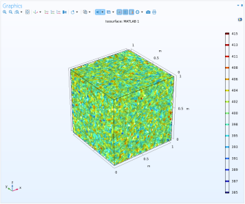
In the Model Builder, under the 3D Plot group 2 node, select the Isosurface 1 node.
6
On the associated Settings page, under the Expression section, enter
conductivity(x)
in the Expression field.
7
Under the Levels section, change the Total levels to
15
.
8
Click the Plot button
.
Note:
The conductivity function has been evaluated again in MATLAB to generate the above plot. As the function is using a random distribution, the plot does not exactly represent the distribution of the thermal conductivity when the solution has been computed.