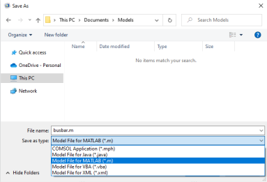
Saving and Running a Model M-File
The easiest way to learn the commands of the COMSOL API is to save a model from the COMSOL Desktop as an M-file. The M-file contains the sequence of commands that create the model. You can open the M-file in a text editor and make modifications to it, as shown in the following example.
Note: By default, the M-file contains the entire command history of the model following the operation done to the model. This means that the model M-file can include settings that are no longer part of the model. In order to include only settings that are part of the current model, compact the model history before saving the M-file. If you want to get the specific command for the last operation that was performed, do not compact the model history.
1
2
3
4
5
6
model.result('pg4').feature('surf1').set('expr', 'ec.normJ');
model.result('pg4').feature('surf1').set('descr', 'Current density norm');
model.result('pg4').feature('surf1').set('rangecolormax', '1e6');
These commands define the plot group pg4, which includes a surface plot of the expression ec.normJ with the maximum color range set to 1e6.
7
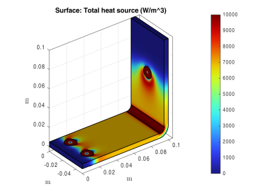
To modify the plot group pg4 so that it displays the total heat jh.Qtot with the maximum color range set to 1e4, add the following lines to the M-file, just before the last command (output of the function):
model.result('pg4').feature('surf1').set('expr','ht.Qtot');
model.result('pg4').feature('surf1').set('descr', 'Total heat source');
model.result('pg4').feature('surf1').set('rangecolormax','1e4');
These commands modify plot group pg4 so that it displays the total heat ht.Qtot with a new setting for the maximum value for the color range. You can also directly modify the original lines corresponding to the plot settings to achieve the same thing, but this way you can easily revert to the old version.
8
9
model = busbar;
10
mphplot(model,'pg4')
Another way to modify a model object in MATLAB is to load the model MPH file in MATLAB, and then enter the commands in step 7 directly at the MATLAB command line. The benefit of this latter approach is that it does not require running the entire model. See An Example Using Nested Loops, where this technique is applied.