Heat Pipe with Accurate Liquid and Gas Properties
Heat pipes are designed to transfer heat efficiently through vaporization, mass transfer, and condensation of a working fluid. They are found in a wide variety of applications where thermal control is of importance, with cooling of electronics being a prominent example.
Inside a heat pipe, the temperature difference between the hot and cold side along with the temperature dependence of the vapor pressure, induce a pressure difference across the vapor chamber. The pressure difference, in turn, drives the vapor from the hot to the cold side. The vaporization acts as a heat sink at the vapor–wick interface at the hot side, and conversely, the condensation as a heat source, at the cold side. This model demonstrates how the laminar flow in the vapor chamber of the heat pipe can be coupled to the liquid phase transport through the porous wick. It also shows how thermodynamic properties of water can be obtained from the database in the Liquid & Gas Properties Module. The importance of vapor transport is compared to the conductive heat transfer in the pipe wall. The former dominates the latter by several orders of magnitude.
Model Definition
Heat pipes exist in variety of different shapes, with tubular ones probably being the most common kind. Here we will look at an axisymmetric model of a copper tube with a porous copper wick and a vapor chamber. The heat pipe has a contact surface at the bottom, which is to be connected to the source of the heat to be removed. At the top of the pipe a similar contact surface for a heat sink is used. The latter often corresponds to a finned metal structure which can easily be cooled by a fan. The geometry used including the different parts is visualized in the figure below.
Overview of the heat pipe geometry.
Before setting up the model, we will investigate under what conditions our assumption of a saturated wick holds.
For heat pipes operating near ambient conditions, the capillary pressure, Δpc, is usually the limiting factor (Ref. 2):
(1)
Here σ is the surface tension and rc is the capillary radius. At the capillary limit, this pressure equals the pressure needed to drive the vapor, the static pressure due to gravity, and the pressure needed to drive liquid through the wick in the manner of:
(2)
For most applications, we can neglect all but the liquid term, which can be obtained from Darcy’s law:
(3)
where μl is the dynamic viscosity of the liquid, Leff is the effective length of the heat pipe, K is the permeability of the wick, Aw is the cross-sectional area of the wick, and is the volumetric flow rate. The latter is governed by the rate of evaporation:
(4)
where, is the heat transfer rate, ρ is the density of the liquid, ΔHvap is the latent heat of vaporization (with dimensionality of energy per mass). Inserting Equation 2-4 into Equation 1, and neglecting Δpv and Δpg yields:
(5)
Evaluating Equation 5 with K =1·10-9 m2, Aw =1·10-4 m2, ΔHvap = 2.5·106J/kg, ρ = 1·103 kg/m3, σ = 7·10-2 N/m, μ = 1·10-3 Pa·s, L = 0.15 m, and r = 3.1·10-5 m, we obtain a value of 7.5 kW. In the model, a modest heat transfer rate of 30 W will be used, thus far from the capillary limit. As a comparison a CPU of a typical consumer PC produces on the order of 10–100 W.
Physics Setup
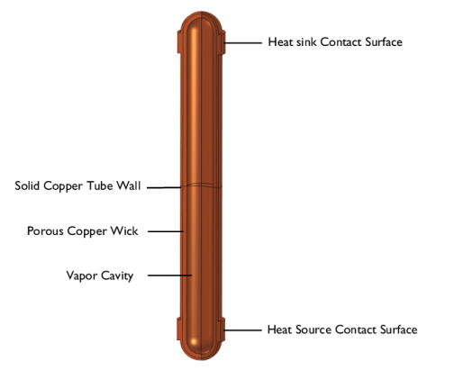
A Laminar Flow interface is used to solve for the flow of fluid in the vapor cavity. It is subject to a single boundary condition, apart from the axial symmetry line. The pressure is prescribed to equal the saturated vapor pressure at the cavity–wick interface.
(6)
This implies that the water and vapor phase are assumed to be in equilibrium at this position. The vapor pressure increases with temperature, which is what drives the vapor from the high temperature region to the low temperature region. For the liquid flow in the porous wick, a Brinkman Equations interface is used. The velocity in the wick at cavity–wick interface is computed from the vapor flow rate on the cavity side
(7)
The pressure level is fixed using a pressure point constraint on the solid wall in the middle of the geometry.
For heat transfer in all parts of the geometry, the tube wall, the wick, and the vapor cavity, a Heat Transfer in Porous Media interface is used. It includes domain features for each domain type.
Material Properties
Material properties are created using the Thermodynamics node. A vapor system using the ideal gas law is set up for the vapor phase, while a liquid system using IAPWS models (Ref. 3) is created for the liquid phase in the wick. To describe the saturation pressure a vapor pressure function is created for the liquid system. In order to easily apply properties in the model, two materials are created using the Generate Material option available for thermodynamic systems. Copper from the material library is used for the properties in the tube wall.
Results and Discussion
As a first step, analyze the temperature when conduction is the only means of energy transport in the pipe. This corresponds to using a dry wick, with no liquid water, and negligible natural convection in the vapor. The resulting temperature is seen in Figure 9 below.
Figure 9: Temperature of heat pipe with dry wick.
We note that the temperature at the heat source is almost 100°C higher than at the heat sink. In an application where temperature sensitive parts are present (electronics, plastics, and so on) such a high temperature would be detrimental.
In the second simulation, the wick is assumed to be saturated with liquid water, corresponding to a heat pipe running at its design point. The resulting temperature profile, seen in Figure 10, looks very different.
Figure 10: Temperature of heat pipe with saturated wick.
The predicted temperature difference between heat sink and heat source is now less than 2°C. And the surface of the heat pipe outside of the contact areas is essentially isothermal. In Figure 11, the computed velocity fields, in both fluids, and the temperature throughout the geometry, are plotted next to each other.
Figure 11: Fluid velocities—lg(|u| / m·s-1) and temperature in the heat pipe running at the design point.
The heat transfer process can be decomposed into different contributions, by computing line integrals across the cavity, wick, and casing at the middle of the pipe. In the table below, the relative importance of the different heat transfer mechanisms in the saturated heat pipe is highlighted.
It is seen that, at normal operating conditions, vapor mass transfer (and its associated phase changes) is the completely dominating mechanism by which the heat pipe transfers heat.
References
2. I. Shishido, I. Oishi, and S. Ohtani, “Capillary Limit in Heat Pipes,” J. Chem. Eng. of Japan, vol. 17, no. 2, pp. 179–186, 1986.
3. W. Wagner and H.J. Kretzschmar IAPWS industrial formulation 1997 for the thermodynamic properties of water and steam. International steam tables: properties of water and steam based on the industrial formulation IAPWS-IF97, pp. 7–150, 2008.
Modeling Instructions: Heat Pipe with Accurate Liquid and Gas Properties
By following the steps described below you will be able to set up a model for a Heat Pipe, analyze it at operating conditions, and see the importance of liquid water in the porous wick.