Tutorial Model — Electronic Chip Cooling
This model is an introduction to simulations of device cooling. A device (here a chip associated to a heat sink) is cooled by a surrounding fluid, air in this case. This tutorial demonstrates the following important steps:
In addition, this tutorial compares two approaches for modeling the air cooling. First, only the solid is represented and a convective cooling heat flux boundary condition is used to account for the heat transfer between the solid and the fluid. In a second step, the air domain is included in the model and a nonisothermal flow model is defined.
Model Definition
The modeled system describes an aluminum heat sink used for the cooling of an electronic chip, as shown in Figure 10.
Figure 10: Heat sink and electronic chip geometry.
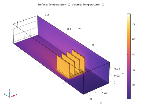
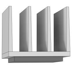
The heat sink represented in gray in Figure 10 is mounted inside a channel with a rectangular cross section. Such a setup is used to measure the cooling capacity of heat sinks. Air enters the channel at the inlet and exits the channel at the outlet. Thermal grease is used to improve the thermal contact between the base of the heat sink and the top surface of the electronic component. All other external faces are thermally insulated. The heat dissipated by the electronic component is equal to 10 W and is distributed through the chip volume.
The cooling capacity of the heat sink can be determined by monitoring the temperature in the electronic component.
The model solves a thermal balance for the electronic component, heat sink, and air flowing in the rectangular channel. Thermal energy is transferred by conduction in the electronic component and the aluminum heat sink. Thermal energy is transported by conduction and advection in the cooling air. Unless an efficient thermal grease is used to improve the thermal contact between the electronic component and the heat sink, the temperature field varies significantly there. The temperature is set at the inlet of the channel. The transport of thermal energy at the outlet is dominated by convection.
Initially, heat transfer by radiation between surfaces is neglected. This assumption is valid as the surfaces have low emissivity (close to 0), which is usually the case for polished metals. In a case where the surface emissivity is large (close to 1), the surface-to-surface radiation should be considered. This is done later in this tutorial, where the model is modified to account for surface-to-surface radiation at the channel walls and heat sink boundaries. Assuming that the surfaces have been treated with black paint, the surface emissivity is close to 1 in this second case.
The flow field is obtained by solving one momentum balance relation for each space coordinate (x, y, and z) and a mass balance equation. The inlet velocity is defined by a parabolic velocity profile for fully developed laminar flow. At the outlet, the normal stress is equal to the outlet pressure and the tangential stress is canceled. At all solid surfaces, the velocity is set to zero in all three spatial directions.
The thermal conductivity of air, heat capacity of air, and air density are all temperature-dependent material properties. You can find all of the settings in the physics interface for Conjugate Heat Transfer in COMSOL Multiphysics. The material properties, including their temperature dependence, are available in the Material Browser.
Results with Convective Cooling Boundary Condition
In this part of the model, only the solid domains are represented. Instead of computing the flow velocity, pressure, and temperature in the air channel, a convective cooling boundary condition is used at the heat sink boundaries. The approach enables very quick computations, but its accuracy relies on the heat transfer coefficient that is used to define the convective cooling condition. In this configuration, an empirical value, 10 W/(m²·K), is used.
Next, to model the thermal contact between the heat sink and the chip three hypotheses are considered. In a first simulation an ideal contact is assumed.
Figure 11: Temperature on half of heat sink surface and on the chip surface assuming perfect thermal contact.
Under ideal conditions, the maximum temperature in the chip is about 85°C.
In the second simulation, a 50-µm-thick layer of air between the heat sink and the chip is assumed to create a thermal resistance.
Figure 12: The surface plot shows the temperature on half of heat sink surface and on the chip surface accounting for a thin air layer between the heat sink and the chip.
The thermal resistance decreases the performance of the heat sink and the maximum temperature is close to 95°C.
Finally, a third configuration is tested where the thin layer contains thermal grease instead of air.
Figure 13: The surface plot shows the temperature on half of heat sink surface and on the chip surface accounting for a thin thermal grease layer between the heat sink and the chip.
The maximum temperature is close to the one observed in the first configuration with an ideal thermal contact. This means that the effect of the thermal resistance is greatly reduced by the thermal grease, which has a higher thermal conductivity than air.
Results with Nonisothermal Flow in the Channel
Since the heat transfer coefficient is in general unknown, an alternative approach is suitable. In this part, a domain corresponding to the air channel is added to the geometry in order to compute the flow and the temperature field in the air. This leads to more computationally expensive simulations, but the approach is more general.
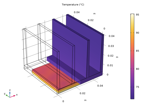
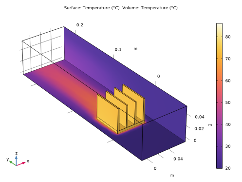
In Figure 14, the hot wake behind the heat sink is a sign of the convective cooling effects. The maximum temperature, reached in the electronic component, is about 85°C.
Figure 14: The surface plot shows the temperature field on the channel walls and the heat sink surface.
Compared with the first approach (without the air domain), the results are different. This shows that using a heat transfer coefficient that is not known with accuracy, as in the first approach, provides good orders of magnitude but can still be approximate.
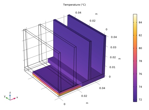
In the second step, the temperature and velocity fields are obtained when surface-to-surface radiation is included and the surface emissivities are large. Figure 15 shows that the maximum temperature, about 75°C, is decreased by about 10 °C when compared to the first case in Figure 14. This confirms that radiative heat transfer is not negligible when the surface emissivity is close to 1.
Figure 15: The effects of surface-to-surface radiation on temperature. The surface plot shows the temperature field on the channel walls and the heat sink surface.